Aims of the chapter

This chapter explores the short- and long-run determinants of unemployment, output and the price level. We begin by describing the labour market and the different components of unemployment, in order to identify appropriate macroeconomic policies to reduce each of them. Next, we derive the aggregate supply (AS) and the aggregate demand (AD) curves and discuss alternative views about the slope of each curve in the short run. The two curves are then combined to form the AD–AS model, which is used to describe business-cycle fluctuations and assess to what extent macroeconomic policy can be employed to stabilise the economy in the short run.

• explain the mechanism underlying the determination of the equilibrium real wage and unemployment rate in the labour market
• recognise the main types and causes of unemployment, and the appropriate macroeconomic policies to reduce them
• derive aggregate supply under imperfect competition in the labour and product markets, and discuss the alternative interpretation of the AS relationship
• compute the aggregate demand curve from the IS–LM model, and clarify the determinants of its slope and position
• employ the AD–AS model in order to assess the determinants of output, the price level and the interest rate over the business cycle
• appraise how monetary and fiscal policy can be used as stabilisation tools in response to demand and supply shocks.

This chapter is divided into two parts. The first part focuses on the labour market under imperfect competition and shows how to determine the equilibrium real wage and natural rate of unemployment. There are four types of unemployment: classical (real wage), frictional (search), structural (mismatch), and cyclical (Keynesian) unemployment. The sum of classical, frictional and structural unemployment determines the so-called natural unemployment rate, which is broadly defined as the average unemployment rate in the medium run. Understanding the alternative components of unemployment is important, as it ultimately allows us to correctly identify appropriate macroeconomic policies to reduce them.

Note that the guide defines as classical the unemployment caused by wage rigidities in the labour market. This is in contrast to frictional unemployment, which is caused by the time necessary to search and find a job, and structural unemployment, which is caused by the mismatch between workers’ needs and skills and job requirements.

The second part of this chapter focuses on the description of the AD–AS model, in order to assess the determinants of output and the price level in the short and the long run. The AS curve is computed from the labour market equilibrium condition, whereas AD is derived from the equilibrium condition in the IS–LM model. Attention is given to the economic theories underpinning the alternative slopes of the AS and the AD curves. Finally, the AD–AS model is employed to explain business-cycle fluctuations, and to assess how monetary and fiscal policy can be used to stabilise the economy in the short run.

It is very important that you are able to analyse the AD and the AS curves both analytically and graphically, and to interpret how changes in any variable or parameter of the two curves will affect their slope or position. Confusion may arise about the slope of the short-run AS curve. In the IS–LM model we took a very simplified view of price stickiness and considered a situation in which prices are fixed. In this context, the short-run AS is represented by a horizontal line in output-price space. However, the appropriate view of price stickiness implies that prices slowly adjust, in the short run, and the AS curve is positively sloped in output–price space. The steepness of the AS curve determines the degree of price rigidity: the flatter the AS curve is, the slower the price adjustment mechanism.

The labour market: main definitions

The labour market includes three categories of individuals: employed, unemployed and inactive. The term employed refers to a person who is currently working. Unemployed refers to a person who is not working and is seeking a job. Inactive denotes a person able to work but not seeking a job. The labour force, L, is the sum of employed, N, and unemployed, U, people, and it is defined analytically as:

L = N + U.

The sum of the labour force and the inactive, I, defines the population of working age PW, as:

PW = L + I = N + U + I.

The unemployment rate u is the ratio between unemployed and the labour force:

u = U/L

whereas the employment rate e is defined as the ratio between employed and the population of working age:

e = N/PW

This shows there is not a one-for-one relationship between changes in the rates of unemployment and employment, as these two variables are connected by the so called participation rate, PR, defined as the ratio between the labour force and the total population of working age:

PR = L/PW

These definitions imply that:

u = 1 − (e /PR)

which shows that an increase in employment reduces the unemployment rate to the extent that it is not offset by a rise in the participation rate. This result is obtained by manipulating the unemployment rate as follows:

u = U/L = (L − N)/L = 1 - (N/L) = 1 - (N/PW)(PW/L) = 1 -e(1/PR)

The empirical evidence shows that the participation rate is not constant over time, but it tends to increase during expansions and to fall during recessions. The latter occurs because when the unemployment rate is high, some unemployed people give up their job search and cannot be counted as unemployed any more. These people are known as discouraged workers, namely people who do not look for work, but who would take work if it was offered to them.

Because workers change their status over time, the labour market can be characterised in terms of worker flows between the three states of employed, unemployed and inactive. A specific unemployment rate can be the outcome of a very active labour market with a high number of separations and hires, or of a stagnant (sclerotic) labour market with relatively few separations and hires. Labour market mobility is measured by the proportion of unemployed leaving unemployment in a specific period of time. The inverse of this measure defines the average duration of unemployment, namely the average length of time people spend in unemployment.

The empirical evidence suggests five basic stylised facts about unemployment. First, the unemployment rate varies across countries and over time. In the US the unemployment rate rose until the mid-1980s, and fell afterwards. In Europe the unemployment rate was relatively low during the 1950s and the 1960s, but it increased over the 1970s and the 1980s, and has been above the US rate over the last 20 years. Second, unemployment is negatively correlated with the business cycle: it sharply increases during recessions and it falls during expansions. Third, the duration in unemployment also varies across countries and over time, and it is correlated with the business cycle. In particular, unemployment duration rapidly increases during recessions, whereas it reduces during economic expansions. Fourth, the proportion of unemployed workers finding jobs is low during downturns when unemployment is high. Finally, the proportion of employed workers losing their jobs is high during recessions when the unemployment rate is high.

In a competitive labour market the equilibrium real wage ensures equality between workers’ labour supply and firms’ labour demand. Panel A in Figure 3.1 describes the labour market in employment-real wage space. The labour force is fixed and indicated by the vertical line L. Labour supply, L S , is positively sloped because workers are ready to substitute leisure for labour as the real wage increases (substitution effect). 1 Labour demand, L D , is negatively sloped because firms demand labour until the marginal product of labour equals the real wage. An increase in the employment level reduces the marginal product of labour, and can be supported in equilibrium only by a corresponding fall in the real wage. The competitive real wage, W CE / P , determines the level of employment N, and, in turn, the level of unemployment U = L – N. In a competitive labour market, the real wage always adjusts to clear any excess of labour supply and/or demand.

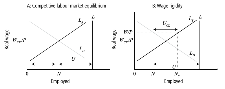
Minimum-wage legislations set a legal minimum compensation that firms must pay to their employees. Minimum wage laws result in a real wage higher than the market clearing wage for those workers with low marginal productivities and equilibrium wages, such as low-skilled and young workers, who tend to receive part of their compensation as job training and apprenticeships. There is an ongoing debate on whether or not minimum wage laws are beneficial for the labour market and the economy as a whole. Supporters argue that minimum wages increase average living standards, create an incentive to work, do not increase public spending, and stimulate consumption by increasing the purchasing power of low-income people who tend to spend their entire wages.

Opponents of minimum wages believe that they ultimately increase unemployment among young or unskilled workers, and should be replaced by income tax credits. Low-income households can deduct the tax credit from their tax payments and, if the credit exceeds the tax bill they can also receive a money refund. The tax credit does not raise firms’ costs and is less likely to deter them from hiring. However, it has the disadvantage of increasing government spending, especially during economic slowdowns.

In many countries wages are the outcome of collective bargaining between unions, firms’ associations and the government. The outcome of the negotiation is known as wage accord, which consists of setting
a specific level for the real wage, then leaving firms free to decide how many workers to hire at this wage. Collective bargaining results in wage rigidities since the power of unions can push the negotiated real wage above the equilibrium wage.

Efficiency wage theories argue that labour productivity is related to worker compensation, and paying a wage above the market-clearing level improves employee morale, thus increasing production. For this reason, firms may be willing to pay a real wage that exceeds the equilibrium wage in order to boost profits. A high wage may also be beneficial for firms in that it reduces the incentive for workers to quit, and thereby the cost of advertising, screening, hiring and training new workers.

The final source of wage rigidity arises from the potential conflict of interest between different groups of workers: insiders and outsiders. Insiders are those workers already employed by firms, who are interested in keeping real wages high. This clearly contrasts with the interest of those unemployed – outsiders – since a wage reduction would increase their chances of employment. A wage rigidity occurs if, within a union, the bargaining power of insiders is greater than that of outsiders, as in this case the insiders can keep the real wage above the equilibrium level.

Hysteresis

Hysteresis in the natural rate of unemployment occurs when the unemployment rate remains very high over a prolonged period of time (persistent unemployment).

Several theories can be advocated to explain this phenomenon. The first view is the human capital decumulation theory. Unemployment reduces both the quality of the labour force (loss of skills) and the attitude of the unemployed towards their likelihood of finding a job (discouragement). Consequently, the quality and quantity of human capital that contributes towards overall production in an economy declines when unemployment is high. This may affect the long-term unemployed, people who have been out of work for long periods of time, and young labour force entrants who lack experience during the formative years of their life.

The second explanation of hysteresis in the natural rate is related to the insider-outsider theory described at the end of the previous section. In essence, when workers become unemployed they are no longer insiders and become outsiders. Consequently, the unemployed do not have any influence on the wage and employment negotiations of the remaining insiders. This prevents the real wage from being reduced enough to increase employment, in turn allowing high unemployment rates to persist over long periods of time.

The third explanation of hysteresis in the natural rate is the physical capital stock theory. This explanation is based on the empirical evidence that high unemployment occurs during economic recessions with very low physical capital formation. If capital and labour are complements in the production function, low capital formation leads to low labour demand, which in turn increases the natural unemployment rate. This is because lower capital stock implies a lower marginal product of labour at any given employment level. Hysteresis in the natural unemployment rate occurs under this theory because after an economic recession it takes a long time to rebuild the capital stock, hence for the full employment level to rise.

Frictional and structural unemployment

The unemployment rate is affected by the degree of mobility in the labour market, which is characterised by people continuously finding and losing jobs. The effect of labour force dynamics on the unemployment rate can be formalised by denoting with l the fraction of employed people losing their jobs in a specific period of time, and with f the share of unemployed people finding a job over the same period of time. If the unemployment rate is constant over the given horizon, and if we assume for simplicity that the participation rate is fixed at 100 per cent then it must be true that:

∆ u = 0 <-> lN = fU ,

which states that a constant unemployment rate over a specific period of time can only occur if the number of employed people losing their jobs equals the number of unemployed people finding new jobs during that period. The definition of labour force, L = N + U, can be substituted into the above to obtain:

l( L − U ) = fU.

After dividing both sides of this expression by L and solving for u, the unemployment rate becomes:

u = 1 / 1 + fl

which shows that the unemployment rate increases as the rate of job finding reduces, or the rate of job losses rises. Equation (3.4) implies that any policy aiming at reducing the steady-state rate of unemployment must either reduce the rate of job losses or increase the rate of job finding. In this context, the unemployment rate can have two very different sources. Frictional unemployment is caused by the time it takes workers to search and find a job. Structural unemployment is instead the outcome of a mismatch between, on the one hand, workers’ needs and characteristics and, on the other hand, vacancy requirements. Factors that determine structural unemployment are job locations, since job vacancies and unemployed people may be located in different regions, and workers’ skills, since workers may be either over- or under-qualified to undertake available jobs. Thus, the longer it generally takes workers to search and find a job, the higher will be frictional unemployment, whereas the higher the degree of mismatch, the higher will be structural unemployment.

The natural rate of unemployment

The natural unemployment rate is defined as the sum of the three components of voluntary unemployment: classical, frictional and structural unemployment. It is a measure of the average or medium-run unemployment rate, around which an economy fluctuates over the business cycle. In the short run, the actual unemployment rate may differ from the natural rate: during expansions the actual unemployment rate is lower than the natural rate, whereas during recessions it is higher. The
difference between the actual and the natural rate of unemployment is defined as cyclical or Keynesian unemployment.

An important way to analyse the natural unemployment rate is by use of the WS–PS model. This requires two modifications to the previous analysis of the labour market. First, the labour market has to be described in unemployment–real wage space. In this space, the labour market is characterised by a decreasing labour supply schedule and an increasing labour demand schedule. Second, imperfect competition is introduced in both the labour and product market, to evaluate how this affects labour
demand, labour supply, and the real wage. In this context, the natural unemployment rate is defined as the equilibrium unemployment rate in a labour market with imperfect competition.

Under imperfect competition, the labour supply curve is replaced by the wage-setting relation, WS, which takes into account the bargaining of workers in wage negotiations, whereas the labour demand curve is replaced by the price-setting relation, PS, which takes into account firms’ power to set the price level above marginal cost.

Blanchard and Johnson provide the following analytical description of the WS and the PS
curves:

WS : W = P^e F ( u , z )
PS : P = ( 1 + μ )W (3.6)

where W indicates the nominal wage, P^e is the expected price level, u is the unemployment rate, z measures structural and institutional factors that contribute to wage determination (i.e. the level of unemployment benefits, labour market protection, minimum wage legislations, etc.) and u is the
markup, which reflects the degree of firms’ market power. The function F is assumed to be decreasing in u, as higher unemployment reduces workers’ ability to bargain for a high real wage.

First, under perfect competition both z and μ equal zero and the WS and the PS curves coincide with the competitive market labour supply and demand curves, respectively. Second, the slope of the PS curve is more generally likely to be positive in unemployment–real wage space. However, the labour market can also be described under an assumption that the marginal product of labour is constant, which results in the PS curve being horizontal. Third, if F(u, z) is linear and equal to 1 + z –
αu, then the WS curve can be written as:

W = Pe (1 + z – αu), (3.6)

where α is the response coefficient of the nominal wage to an increase in unemployment.

The WS–PS model can be employed to compute, analytically, the natural rate of unemployment u_n To this end, note that the natural unemployment rate is a medium-term concept, which holds when P = P e . That is it is calculated under the assumption that price expectations turn out to be
correct. Under this assumption, the nominal wage in equation (3.5) can be replaced with the nominal wage in equation (3.6) to obtain:

1 = ( 1 + z − α u_n ) ( 1 + μ )

This expression can be solved for the natural unemployment rate u_n as follows:

u_n = μ+z (l+μ)/α(l+μ)

which shows that increases in both z and μ raise the natural unemployment rate. If μ is close to zero then this is well approximated by:

u n ≅ μ + z/ α

The concept of a natural unemployment rate implies natural levels of employment and output. The natural level of employment, Nn , is given by:

Nn = L(1 – un )

If output is produced according to the production function: Y = AN,

where A indicates the level of technology, then substitution of the natural level of employment into the production function gives the natural level of output:

Y n = AN n = AL(1 – u n )

Aggregate supply

The AS relation describes how the price level adjusts over time in response to changes in aggregate demand and income.

There are several approaches to the determination of the AS curve. Blanchard and Johnson combine the WS and the PS curves and solves for the price level. This yields the AS curve in equation (7.2) of Blanchard and Johnson’s textbook. 3 This expression looks quite different from the more compact form for the AS curve used by Dornbusch et al. and Mankiw, which is written as:

P = P^e + λ [ Y − Y_n ] (3.9a)

This equation states that the deviation of the actual price level from the expected price level, P – P^e , is proportional to the deviation of output from its natural level, Y – Y n . The definition of the natural level of unemployment implies that along the AS curve the price level equals its expected value, P = P^e, when output equals its natural level, Y = Y_n . If the current level of output exceeds the natural level, Y > Y_n , then the current price level exceeds its expected level, P > P^e .

Alternatively, the AS relation can also be solved for output to obtain the so-called surprise-supply relation: Y = Y n + μ(P – P^e ), where μ = 1/λ > 0 and the term P – P^e indicates surprise inflation. This relation shows that output exceeds the natural level to the extent that there is surprise inflation in the economy (i.e. the actual price level exceeds the expected one).

The parameter λ in equation (3.9a) measures the slope of the AS curve, namely how quickly the price level changes in response to variations in the output gap.

There are three possible scenarios, as illustrated in the first three panels of Figure 3.2. Under the assumption of the IS–LM framework prices are fixed and the AS curve is horizontal (panel A). In the long run (more than 5–10 years) prices are fully flexible and the AS curve is vertical at the natural level of output (panel B). This is because the long-run equilibrium, in the labour market, is defined in real terms, and changes in the price level have no effect on the natural rate of unemployment, and thus the natural level of output. The long-run AS curve is denoted in the guide as LRAS. In the short run, nominal rigidities, and/or imperfect information, make the AS curve positively sloped (panel C). The short-run aggregate supply curve is denoted in the guide as SRAS.

The position of the SRAS curve is determined by all the factors that contribute to equilibrium in the labour market. In particular, an increase in the expected price level makes workers bargain for higher wages (for any given unemployment rate). The increase in the wage raises the actual price that firms set. As a result, an increase in the expected price level causes the AS curve to shift upwards (Figure 3.2, panel D).

The AS relation in equation (3.9a) shows that the extent to which output deviates from its natural level for any given deviation of prices from expectations depends upon the steepness of the SRAS, as determined by the magnitude of the coefficient λ. The smaller is λ, the more variable output becomes relative to prices. There are four theories that explain why output may deviate from its natural level in the short run: the sticky-wage model, the worker-misperception model, the sticky-prices model, and the imperfect information or Lucas ‘islands’ model. It is important that you note how each theory explains the positive slope of the AS curve as a result of a market imperfection: the sticky-wage and the worker-misperception models focus on imperfections in the labour market, whereas the sticky-prices and the imperfect information models focus on imperfections in the product market.

The sticky-wage model

The sticky-wage model is grounded upon two assumptions. First, nominal wages are sticky in the sense they cannot adjust quickly when the economic conditions change, since they are fixed over long periods of time. Second, collective bargaining determines only the level of the nominal wage, whereas employment is determined by firms’ labour demand, because workers agree to provide as much labour as the firms wish to buy at the predetermined wage. This implies that, once the real wage has been set according to the expected price level, then an increase in the price level above the expected value leads to a fall in the real wage and increases labour demand. In turn, the increase in employment raises output, at least until the next wage negotiation. Analytically, the sticky-wage model is described by three equations:

Actual real wage: W/P = W/P^e × P^e/P ;
Labour demand: N − N_n = -((W/P)-(W/P^e);
Output: Y – Y_n = A(N–N_n).

The first equation shows that the actual real wage W/P deviates (above or below) from the predetermined real wage W/P^e to the extent that the expected price level differs (lower or higher) from the actual price level, P^e /P. The second equation shows that labour demand is inversely related to the real wage. An increase in the price level above the expected level increases employment, as it reduces real wages. The final equation shows that output is above the natural level to the extent that firms hire a number of workers higher than the natural employment level.

The sticky-wage model predicts that if after the negotiation the actual price level equals the expected price level, P = P^e , then employment equals its natural level, N = N_n , and consequently output equals its natural level, Y = Y_n . If, however, after the wage negotiation the price level is higher than the expected one, P – P^e > 0, then it must be true that output exceeds its natural level, Y – Y_n > 0, since firms can employ a number of workers in excess of the natural employment level, N – N_n > 0, at least until the next wage negotiation. Vice versa, an unexpected fall in the price level raises the real wage, making labour more expensive. The higher real wage induces firms to reduce employment, and the reduced employment leads to a fall in output. When contracts are renegotiated, workers accept lower nominal wages to restore the original real wage, so employment rises. Therefore, the sticky-wages model predicts that the longer the period over which wages are negotiated, the flatter the SRAS. In addition, the model predicts that real-wage fluctuations are negatively related to output fluctuations.

The worker-misperception model

The worker-misperception model assumes that wages are fully flexible, unlike the sticky-wage model, but workers have imperfect information, in that they suffer from money illusion, so they temporarily
mistake nominal wage increases for real wage increases. Firms have perfect information and their demand for labour depends on the actual real wage, which is written as:

L_D = L_D (W/P)

Analytically, the supply of labour is described as:

L^S = L^S (W/P^e ),

which shows that the quantity of labour supplied by workers depends upon their expected real wage. This can also be written as:

W/P^e = (W/P)(P/P^e)

which shows that the expected real wage is given by the product between the actual real wage and the misperception ratio P/P^e . If (P/P^e ) >1 the actual price level is higher than expected. Vice versa, (P/P^e ) < 1 the actual price level is lower than expected. The expression for the expected real wage can be substituted into the labour supply curve to obtain:

L^S = L^S((W/P)(P/P^e)

which shows that labour supply depends upon the degree of workers’ misperception of the price level P. Consequently, the position of the economy following an increase in P depends upon whether or not workers anticipate the increase in the price level. If they do, then (P/P^e ) = 1: neither labour supply nor labour demand change. The nominal wage rises proportionally with the price level so that real wage, unemployment and output remain unchanged.

If workers fail to anticipate the price-level increase, then firms can offer higher nominal wages which workers mistake for higher real wages. This causes an increase in labour supply, and allows firms to temporarily raise output above the equilibrium level, at least until workers realise that the real wage has not risen, so they revise their expectations and reduce labour supply.

The worker-misperception model implies an AS curve that is positively sloped in the short run. In particular, for given price expectations the more elastic are the labour supply and demand schedules, the flatter will be the SRAS.

The sticky-price model

The sticky-price model assumes that some firms cannot quickly change prices as a result of variations in aggregate demand, because it is costly to alter prices once they have been published in catalogues, menus and price lists (menu costs). In particular, the aggregate price level can be analytically described as:

P = sP^e + ( 1 − s ) [ P+ α ( Y − Y_n ) ],

where 0 ≤ s ≤ 1 is the share of firms with sticky prices setting the price level according to their expectations; (1 – s) is the share of flexible price firms, which can immediately change the price level in response to an increase in demand above the natural level of output; and α > 0 is the
response coefficient of flexible prices to demand. If we first subtract P(1–s) from both sides of the above and then divide by s, the price level under the sticky-price model becomes:

P = P^e + ((1-s)α/s)(Y - Y_n)

This equation shows two features of the sticky-price model. First, a high expected price level leads to a high actual price level; since firms that set the price in advance expect a high price level, they will set high prices in order to face future high costs. These high prices cause all other firms also to set high prices. Second, the effect of changes in output on the price level depends upon the proportion of firms with flexible prices, as measured by the parameter (1 – s)/s. The lower s is, the steeper the SRAS, since deviations of output from its natural level cause a greater share of firms to
change their prices.

Aggregate demand

The AD relation defines combinations of the price level and income such that the goods and money markets are simultaneously in equilibrium. Analytically, the AD relation is obtained by substituting into the equation for the IS curve the equilibrium interest rate determined from the LM curve. 5 Using the IS and the LM curve defined in equations (2.11) and (2.12) in Chapter 2 of the subject guide, the AD relation can be written as:

This is a very generic and (apparently) complicated expression. However, if you set m = [ 1 − c 1 ( 1 − τ 1 ) − b 1 ] to indicate the parameters of the multiplier and A= ( c 0 − c 1 T + I + G ) to denote the level of autonomous spending, then the AD curve can be written in the more compact form:

which can be further rearranged as:

(3.12)

Equation (3.12) gives the basic equation for the AD curve in a closed economy. There are several things that you may want to bear in mind at this stage.

First, note that in equation (3.12), unlike equation (2.12) in Chapter 2, the price level is not fixed. The AD curve evaluates the goods and money market equilibrium conditions in the short run, during which prices are sticky but not entirely fixed.

Second, equation (3.12) shows that the position of the AD curve depends on the level of autonomous spending, and it is generally affected by fiscal policy and monetary policy (T, G, M, τ1 ) and private sector behaviour, as summarised by the parameters c0 , c1 , b1 , b2 , h1 and h2 . In particular, fiscal and monetary expansions shift the AD curve upwards, as they increase equilibrium income in the IS-LM model. Conversely, fiscal and monetary contractions shift the AD curve downwards.

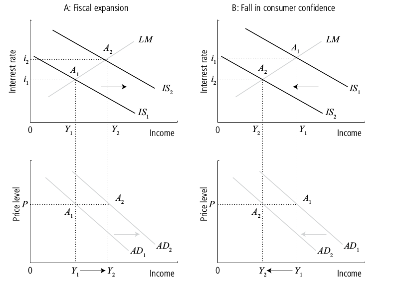
Figure 3.3 displays the link between the IS–LM model and the AD curve. Panel A shows that a fiscal expansion shifts the IS curve to the right, thus increasing the equilibrium level of income from Y 1 to Y 2 . At any price level P, the AD curve shifts horizontally, to the right, by the same increase in output implied by the IS–LM model. Panel B shows that a reduction in consumer confidence – as measured by the parameter c 0 – shifts the AD curve to the left, so that the reduction in income at any price level P in the AD diagram is equal to the reduction in the equilibrium level of income observed in the IS–LM diagram.

Finally, it is important that you have a clear understanding of the theoretical explanations provided for the negative slope of the AD curve. To this end remember that the AD curve is derived from the simultaneous equilibrium in the goods and the money markets. The variable that links these two market
is the interest rate, which affects investment in the goods markets, through the parameter b2 , and money demand in the money market, through the parameter h2 . In general this results in a negatively-sloped AD curve because of the Keynes effect: when the price level rises the value of

M^S/P

falls. In order for the money market to clear, the opportunity cost of holding money must then rise – that is, the interest rate must increase. The increase in the interest rate reduces demand for investment and, in turn, output.

There are two situations in which this mechanism fails to work. In both cases, the AD curve is vertical. The first case occurs when investment does not respond to changes in the interest rate, (i.e. b 2 = 0). The AD curve is vertical because, in this case, the increase in the interest rate due to a rise in the price level is not transmitted to output, as demand for investment does not respond to changes in the interest rate. Consequently, output does not change as the price level changes. The AD curve is also vertical when the economy is in a liquidity trap (i.e. h 2 = ∞). In this case, a rise in the price level still reduces real money balances. However, this has no effect on this
interest rate because the demand for real money balances is perfectly elastic. Thus variations in the price level have no effect on investment and output.

Yet even in these extreme cases it has been argued that the AD curve may have a negative slope. This is because of the so-called Pigou or wealth or real balances effect. Suppose the level of consumption itself depends upon the level of real balances. Then when the price level increases, the real value of money falls, in turn reducing consumer spending and output. As a result, a change in the price level will have a direct effect on aggregate demand, through consumption. In particular, an increase
in real money balances due to a reduction in prices causes a rightward shift in the IS curve, alongside the usual downward shift of the LM curve. To the extent that consumption depends upon real balances, the Pigou effect compounds the Keynes effect. Consequently, the AD curve is flatter with the Pigou effect than under the Keynes effect alone. In addition, under the Pigou effect the AD curve is negatively sloped regardless of the sensitivity of investment and money demand to changes in the interest rate. Therefore, with the addition of the Pigou effect, the AD curve cannot be vertical.

The AD–AS model

The AD and the AS relations can be employed to determine the general equilibrium in the economy, namely the price and output levels that simultaneously clear the goods, the money and the labour markets. In the short run equilibrium occurs when the AD curve equals the SRAS. This may occur at any price and output level. In the long run, the economy is in equilibrium when the AD curve equals the LRAS. Because in the long run output is fixed at its natural level, the long-run equilibrium is consistent with any price level along the LRAS.

The short-run equilibrium condition determines the actual price level as well as the actual level of output, whereas the long-run equilibrium condition determines the long-run price level alone, since long-run output is determined within the labour market. In the short run, the actual price
level normally differs from the expected level. For this reason, the short-run equilibrium is not stable over time, and output adjusts until P = P^e . More precisely, if the actual price level exceeds the expected one, wage setters increase their wage demands as their price expectations increase, which in turn shifts the SRAS upwards. This process of medium-run adjustment continues until the SRAS equals the AD curve at P = P^e (i.e. until the economy reaches the long-run equilibrium).

The important thing to note at this stage is that the economy has a built-in adjustment mechanism, so that output returns, sooner or later, to its natural level once either a negative or a positive shock hits the economy.

Monetary and fiscal policy in the AD–AS model

The AD–AS framework is, mostly, employed to assess the effectiveness of macroeconomic policy as a tool to stabilise the economy over the business cycle. A first important prediction of the model is known as classical dichotomy, which states that in the long run all real variables in the economy, such as aggregate real output, unemployment and real wages, are determined independently of monetary policy, which can only affect the long-run price level. Consequently, the AD–AS model predicts that in the long run monetary policy is neutral, in the sense that it can only alter output, unemployment and the interest rate in the short run. In the long run a monetary expansion results in an increase in the equilibrium price level alone, since the increase in the price level fully offsets the initial
nominal money supply expansion.

In the short run, monetary policy can still affect cyclical unemployment: long-run neutrality does not imply that monetary policy is useless. A monetary expansion increases output and reduces the interest rate in the short run, therefore it can be successfully employed to speed up the recovery from a recession. Moreover, by reducing more quickly cyclical unemployment, an expansionary monetary policy can also, indirectly, influence the natural unemployment rate, by limiting the increase in
unemployment due to hysteresis arising from the dependence of the natural unemployment rate on the history of cyclical fluctuations.

The AD–AS model predicts that, in contrast with monetary policy, fiscal policy is non-neutral, as it affects the long-run equilibrium interest rate and thus demand for investment. A fiscal contraction reduces both output and the price level in the short run. Contemporaneously, the fall in the price level increases the real money supply, in turn reducing the equilibrium interest rate in the money market. This is compounded by the usual reduction in interest rates that follow a fiscal contraction in the IS–LM model. The result is an increase in the demand for investment, offsetting some of the fall in output. In the long run the fiscal contraction has no aggregate effect on output, which returns to its natural level as price expectations adjust. But the effect on investment remains: it has filled the gap left by lower government expenditure.

The AD–AS model suggests that macroeconomic policy can be effectively employed as a tool for economic stabilisation (demand management or fine-tuning policy). Macroeconomic fluctuations can be regarded as the outcome of demand (IS and LM) shocks, namely unexpected changes in the private sector demand for consumption and investment. These shocks cause output to deviate, temporarily, from its natural level, and the actual price level to differ from the expected level. As discussed at the end of the previous section, the market already has an adjustment mechanism which tends to stabilise the economy in the medium run. However, monetary and fiscal policy can be employed to accelerate the medium run adjustment and, therefore, reduce macroeconomic fluctuations.

Finally, the magnitude of demand shocks, and, in turn, the effectiveness of macroeconomic policy as a stabilisation tool in the short run, ultimately depend upon the degree of price flexibility, as
represented by the slope of the SRAS. In principle, if prices are extremely flexible (SRAS relatively steep) macroeconomic actions are relatively ineffective, but the effects of demand shocks will also be less problematic as the economy is able to adjust quickly on its own. In contrast, the flatter the
SRAS is, the greater the destabilising effects of macroeconomic shocks, and also the greater the effectiveness of macroeconomic policy as a stabilisation tool.

Supply shocks

Supply shocks are unexpected changes in the position of the AS curve. A negative supply shock, such as an increase in the price of oil or other raw materials, increases the price level for any value of output. A positive supply shock, such as the discovery of a new and more efficient production technology, reduces the price level for any level of output.

i. how supply shocks may affect the economy over the business cycle, and
ii. to what extent macroeconomic policy can (and should) be employed in response to supply shocks.

Panel A in Figure 3.4 describes a (permanent) negative supply shock. The economy is initially in equilibrium at point A, where output equals the natural level Yn,1 , the actual price level P1 corresponds with the expected price level Pe1 , and the interest rate – in the IS–LM diagram – equals i1 . The negative supply shock increases firms’ production costs, inducing them to set higher prices. This results in the SRAS shifting upwards from SRAS 1 to SRAS 2 . Contemporaneously, in the labour market the PS curve falls down, reflecting lower labour productivity which results in a permanent
increase in the natural unemployment rate. The increase in the natural unemployment rate leads to a fall in the natural level of output to Y n,3 , with the LRAS shifting to the left from LRAS 1 to LRAS 3 . The new short-run equilibrium is at point B, which entails higher output relative to the new long-run level, Y 2 > Y n,3 , and a new price level P 2 which is higher than the expected price level P e 1 . The SRAS begins to shift upwards until it reaches the new long-run equilibrium at C. Contemporaneously, in the IS–LM diagram the increase in the price level reduces real money balances, and the LM curve shifts upwards until it reaches the new equilibrium position at C. In sum, a negative supply shock reduces output, increases the price level, and raises the interest rate.

Panel B in Figure 3.4 describes a (permanent) positive supply shock. The economy is initially in equilibrium at point A, where output equals the natural level Y n,1 , the actual price level P 1 corresponds with the expected price level P e 1 , and the interest rate – in the IS–LM diagram – equals i 1 . The positive supply shock reduces firms’ production costs, causing a lower aggregate price level to be set. This results in the SRAS shifting downwards from SRAS 1 to SRAS 2 . Contemporaneously, in the labour market the PS curve shifts upwards, resulting in a permanent fall in the natural unemployment rate. The reduction in the natural unemployment rate leads to an increase in the natural level of output to Y n,3 , with the LRAS shifting to the right from LRAS 1 to LRAS 3 . The new short-run equilibrium is at point B, which entails lower output relative to the new long-run level, Y 2 < Y n,3 , and a new price level P 2 which is lower than the expected price level P e 1 . The SRAS begins to shift downwards until it reaches the new long-run equilibrium at C. Contemporaneously, in the IS–LM diagram, the fall in the price level raises real money balances and the LM curve shifts downwards until it reaches the new equilibrium position at C. Therefore, a positive supply shock increases output, reduces the price level and decreases the interest rate.

Note that, in general, the AD and the IS curves are also likely to respond to supply shocks. An increase in the price of oil may lead firms to reduce demand for investment and may also determine a fall in consumption, as it redistributes income from oil consumers to oil producers. Public spending
may also be affected as governments may decide to increase investment in energy-efficient projects or pursue investment in alternative sources of energy. Positive supply shocks are also likely to affect the AD and the IS curves, even though this depends on the source of the shock. On the one hand, a shock resulting in a widespread diffusion of new discoveries and inventions increases the likely rate of future growth, and, in turn, raises consumer and business confidence. This type of shock is likely to increase current consumption and demand for investment, and thus to cause a rightward shift in the IS and AD curves. In contrast, a positive supply shock due to a new technology that makes firms more efficient may lead to a fall in labour demand, and undermine consumer confidence. As a result, both
the IS and AD curves would shift to the left.

An important question is whether, and to what extent, macroeconomic policy can be used in response to supply shocks. Positive supply shocks increase output and reduce the price level, which is not regarded as a negative outcome, as most people like higher output and lower prices. The issue is
more complicated for negative supply shocks, since they lead to stagflation, that is a period of economic recession accompanied by an increase in the price level. Fiscal or monetary expansions would help the recovery of output, but also further increase the price level. Vice versa, fiscal and monetary contractions would contribute to reducing the price level, but would further depress output.

Blanchard, O. and D.R. Johnson Macroeconomics. (Upper Saddle River, NJ: Prentice Hall, 2018

Chapter 5

• Output and prices are determined by aggregate supply and aggregate demand.
• In the short run, the aggregate supply curve is flat. In the long run, the aggregate supply curve is vertical. It is upward sloping in the medium run.
• The aggregate supply curve describes the price adjustment mechanism of the economy.
• Changes in aggregate demand, the result of changes in fiscal and monetary policy as well as individual decisions about consumption and investment, change output in the short run and change prices in the long run.

The aggregate supply–aggregate demand model is the basic macroeconomic tool for studying output fluctuations and the determination of the price level and the inflation rate. We use this tool to understand why the economy deviates from a path of smooth growth over time and to explore the consequences of government policies intended to reduce unemployment, smooth output fluctuations, and maintain stable prices.

The aggregate supply (AS) curve describes, for each given price level, the quantity of output firms are willing to supply. The AS curve is upward-sloping because firms are willing to supply more output at higher prices. The aggregate demand (AD) curve shows the combinations of the price level and level of output at which the goods and money markets are simultaneously in equilibrium. The AD curve is downward-sloping because higher prices reduce the value of the money supply, which reduces the demand for output. The intersection of the AD and AS schedules ... determines the equilibrium level of output, Y_0 , and the equilibrium price level, P_0 . Shifts in either schedule cause the price level and the level of output to change.

The aggregate supply curve describes, for each given price level, the quantity of output firms are willing to supply. In the short run the AS curve is horizontal (the Keynesian aggregate supply curve); in the long run the AS curve is vertical (the classical aggregate supply curve).

The classical aggregate supply curve is vertical, indicating that the same amount of goods will be supplied whatever the price level. The classical supply curve is based on the assumption that the labor market is in equilibrium with full employment of the labor force. If the idea that the aggregate supply curve is vertical in the long run makes you uncomfortable, remember that the term “price level” here means overall prices.

The Keynesian aggregate supply curve is horizontal, indicating that firms will supply whatever amount of goods is demanded at the existing price level. The idea underlying the Keynesian aggregate supply curve is that because there is unemployment, firms can obtain as much labor as they want at the current wage... In truth, even in the very short run, the aggregate supply curve has a very slight upward tilt. But in building models we always make simplifying approximations.

It is important to note that on a Keynesian aggregate supply curve, the price level does not depend on GDP.

The natural rate of unemployment is the rate of unemployment arising from normal labor market frictions that exist when the labor market is in equilibrium.

The aggregate supply curve describes the price adjustment mechanism of the economy... Think of the aggregate supply curve as rotating, counterclockwise, from horizontal to vertical with the passage of time.... Tomorrow’s price level equals today’s price level if, and only if, output equals potential output. 4 The difference between GDP and potential GDP, Y - Y * , is called the GDP gap, or the output gap .

We summarize the description of the aggregate supply schedule as follows:
* A relatively flat aggregate supply curve means that changes in output and employment have a small impact on prices.
* The position of the short-run AS schedule depends on the level of prices.
* The short-run AS schedule shifts over time. If output is maintained above the full-employment level, Y^* , prices will continue to rise over time.

In a recession we are on the flat part of the aggregate supply curve, so demand management policies can be effective at boosting the economy without having much effect on the price level. However, as the economy approaches full employment, policymakers must be wary of too much stimulus to avoid running the aggregate demand curve up the vertical portion of the aggregate supply curve.

The aggregate demand curve shows the combinations of the price level and level of output at which the goods and money markets are simultaneously in equilibrium. Expansionary policies ... move the aggregate demand curve to the right. Consumer and investor confidence also affects the aggregate demand curve. When confidence increases, the AD curve moves to the right. When confidence drops, the AD curve moves to the left.

The key to the aggregate demand relation between output and prices is that aggregate demand depends on the real money supply. The real money supply is the value of the money provided by the central bank and the banking system. If we write the number of dollars in the money supply (the nominal
money supply ) as barM and the price level as P, we can write the real money supply as barM/P. When barM/P rises, interest rates fall and investment rises, leading overall aggregate demand to rise. Analogously, lowering barM/P lowers investment and overall aggregate demand.

For a given level of the nominal money supply, barM , high prices mean a low real money supply, barM/P. Quite simply, high prices mean that the value of the number of available dollars is low. As a result, a high price level means a low level of aggregate demand, and a low price level means a high level of aggregate demand.

The quantity theory of money provides a simple way to get a handle on the aggregate demand curve, even if it does leave out some important elements. The total number of dollars spent in a year, nominal GDP , is P * Y. We call the number of times per year a dollar turns over velocity , V . If the central bank provides M dollars, then: M * V = P * Y.

If we make one additional assumption—that V is constant—then equation (2) turns into an aggregate demand curve. With the money supply constant, any increase in Y must be offset by a decrease in P , and vice versa.

It is important for what follows to see that an increase in the nominal money stock shifts the AD schedule up exactly in proportion to the increase in nominal money.

We have repeatedly used the terms “Keynesian” and “classical” to describe assumptions of a horizontal or vertical aggregate supply curve. Note that these are not alternative models providing alternative descriptions of the world. Both models are true: The Keynesian model holds in the short run, and the classical model holds in the long run. Economists do have contentious disagreements over the time horizons in which either model applies. Almost all economists ( almost all) agree that the Keynesian model holds over a period of a few months or less and the classical model holds when the time frame is a decade or more. Unfortunately, the interesting time frame for policy relevance is several quarters to a few years.

All economists are in favor of policies that move the aggregate supply curve to the right by increasing potential GDP. Such supply-side policies as removing unnecessary regulation, maintaining an efficient legal system, and encouraging technological progress are all desirable, although not always easy to implement. However, there is a group of politicians and pundits who use the term “supply-side economics” in reference to the idea that cutting tax rates will increase aggregate supply enormously—so much, in fact, that tax collections will rise, rather than fall.

Cutting tax rates has effects on both aggregate supply and aggregate demand. The aggregate demand curve shifts right from AD to AD^1. The shift is relatively large. The aggregate supply curve also shifts to the right, from AS to AS^1, because lower tax rates increase the incentive to work. However, economists have known for a very long time that the effect of such an incentive is quite small, so the rightward shift of potential GDP is small. ... In the short run, the economy moves from E to E^1. GDP does rise substantially. As a result, total tax revenues fall proportionately less than the fall in the tax rate. However, this is purely an aggregate demand effect. In the long run, the economy moves to E^2. GDP is higher, but only by a very small amount. As a result, total tax collections fall and the deficit rises. In addition, prices are permanently higher. The United States experimented with supply-side economics in the 1981–1983 tax cuts. The results were just as predicted. Not all supply-side policies are silly. In fact, *only* supply-side policies can permanently increase output. Important as they are, demand management policies are useful only for short-term results. Many conservative economists favor cutting tax rates for the small, but real, incentive effect. However, these economists also believe in cutting government spending at the same time. Tax collections would fall, but so would government spending, so the effect on the deficit
would be nearly neutral.

The long-run aggregate supply curve marches to the right over time at a fairly steady rate. Two percent annual growth is pretty low, and 4 percent is high. In contrast, movements in aggregate demand over long periods can be either large or small, depending mostly on movements in the money supply.

1. The aggregate supply and demand model is used to show the determination of the equilibrium levels of both output and prices.
2. The aggregate supply schedule, AS , shows at each level of prices the quantity of real output firms are willing to supply.
3. The Keynesian supply schedule is horizontal, implying that firms supply as many goods as are demanded at the existing price level. The classical supply schedule is vertical. It would apply in an economy that has full price and wage flexibility. In such a frictionless economy, employment and output are always at the full-employment level.
4. The aggregate supply curve describes the dynamic price adjustment mechanism of the economy.
5. The aggregate demand schedule, AD , shows at each price level the level of output at which the goods and assets markets are in equilibrium. This is the quantity of output demanded at each price level. Along the AD schedule fiscal policy is given, as is the nominal quantity of money.
6. A fiscal expansion shifts the AD schedule outward and to the right. An increase in the nominal money stock shifts the AD curve up by the same proportion as the money stock increases.
7. Supply-side economics makes the claim that reducing tax rates generates very large increases in aggregate supply. In truth, tax cuts produce very small increases in aggregate supply and relatively large increases in aggregate demand.
8. Over long periods, output is essentially determined by aggregate supply and prices are determined by the movement of aggregate demand relative to the movement of aggregate supply.

Blanchard, O., Johnson, D.R., (2013) Macroeconomics (sixth edition), Pearson

Chapter 6: The Labor Market

Think about what happens when firms respond to an increase in demand by increasing production: Higher production leads to higher employment. Higher employment leads to lower unemployment. Lower unemployment leads to higher wages. Higher wages increase production costs, leading firms to increase prices. Higher prices lead workers to ask for higher wages. Higher wages lead to further increases in prices, and so on.

So far, we have simply ignored this sequence of events: By assuming a constant price level in the IS–LM model, we in effect assumed that firms were able and willing to supply any amount of output at a given price level. So long as our focus was on the short run, this assumption was acceptable. But, as our attention turns to the medium run, we must now abandon this assumption, explore how prices and wages adjust over time, and how this, in turn, affects output.

...economists sometimes focus on the employment rate, the ratio of employment to the population available for work, rather than on the unemployment rate. The higher unemployment, or the higher the number of people out of the labor force, the lower the employment rate.

We capture our discussion of wage determination by using the following equation:
W = P^e F(u, z) (expected price level, unemployment, disturbance term

An increase in the unemployment rate decreases wages.

Having looked at wage determination, let’s now turn to price determination. The prices set by firms depend on the costs they face. These costs depend, in turn, on the nature of the production function—the relation between the inputs used in production and the quantity of output produced—and on the prices of these inputs.

Y = AN

where Y is output, N is employment, and A is labor productivity. This way of writing the production function implies that labor productivity—output per worker—is constant and equal to A.

If there were perfect competition in the goods market, the price of a unit of output would be equal to marginal cost: P would be equal to W . But many goods markets are not competitive, and firms charge a price higher than their marginal cost. A simple way of capturing this fact is to assume that firms set their price according to

P = (1 + m)W

where m is the markup of the price over the cost. If goods markets were perfectly competitive, m would be equal to zero, and the price P would simply equal the cost W . To the extent they are not competitive and firms have market power, m is positive, and the price P will exceed the cost W by a factor equal to (1 + m).

P/W = 1 + m

W/P = 1/1+m

Price-setting decisions determine the real wage paid by firms. An increase in the markup leads firms to increase their prices given the wage
they have to pay; equivalently, it leads to a decrease in the real wage.

The natural rate of unemployment is the unemployment rate such that the real wage chosen in wage setting is equal to the real wage implied by price setting.

Equilibrium in the labor market requires that the real wage chosen in wage setting be equal to the real wage implied by price setting.

a better name for the equilibrium rate of unemployment would be the structural rate of unemployment, but so far the name has not caught on.

* The real wage chosen in wage setting is a decreasing function of the unemployment rate.
* The real wage implied by price setting is constant.
* Equilibrium in the labor market requires that the real wage chosen in wage setting be equal to the real wage implied by price setting. This determines the equilibrium unemployment rate.
* This equilibrium unemployment rate is known as the natural rate of unemployment.
* Associated with the natural rate of unemployment is a natural level of employment and a natural level of output.

Chapter 7: Putting All Markets Together: The AS–AD Model

The aggregate supply relation captures the effects of output on the price level. It is derived from the behavior of wages and prices W = P^e F(u, z).

A better name would be “the labor market relation.” But because the relation looks graphically like a supply curve (there is a positive relation between output and the price), it is called “the aggregate supply relation.”

The AS relation has two important properties:
The first property is that, given the expected price level, an increase in output leads to an increase in the price level. This is the result of four underlying steps:

1. An increase in output leads to an increase in employment.
2. The increase in employment leads to a decrease in unemployment and therefore to a decrease in the unemployment rate.
3. The lower unemployment rate leads to an increase in the nominal wage.
4. The increase in the nominal wage leads to an increase in the prices set by firms and therefore to an increase in the price level.

The second property is that, given unemployment, an increase in the expected price level leads, one for one, to an increase in the actual price level. For example, if the expected price level doubles, then the price level will also double. This effect works through wages:

1. If wage setters expect the price level to be higher, they set a higher nominal wage.
2. The increase in the nominal wage leads to an increase in costs, which leads to an increase in the prices set by firms and a higher price level.

If output is equal to the natural level of output, the price level is equal to the expected price level.

The aggregate supply curve is upward sloping. Put another way, an increase increase in output Y leads to an in the price level P.

The aggregate supply curve goes through point A, where Y = Y^n and P = P^e . Put another way: When output Y is equal to the natural level of output Y^n , the price level P turns out to be exactly equal to the expected price level P^e . High economic activity puts pressure on prices.

* Starting from wage determination and price determination in the labor market, we have derived the aggregate supply relation.
* This relation implies that for a given expected price level, the price level is an increasing function of the level of output. It is represented by an upward-sloping curve, called the aggregate supply curve.
* Increases in the expected price level shift the aggregate supply curve up; decreases in the expected price level shift the aggregate supply curve down.

The aggregate demand relation captures the effect of the price level on output. It is derived from the equilibrium conditions in the goods and financial markets.

Equilibrium in the goods market requires that output equal the demand for goods—the sum of consumption, investment, and government spending. This is the IS relation. Equilibrium in financial markets requires that the supply of money equal the demand for money. This is the LM relation. Using the IS and LM relations, we can derive the relation between the price level and the level of output implied by equilibrium in the goods and financial markets.

A better name would be “the goods market and financial markets relation.” But, because it is a long name, and because the relation looks graphically like a demand curve (that is, a negative relation between output and the price), it is called the “aggregate demand relation.”

An increase in the price level leads to a decrease in the real money stock. This monetary contraction leads to an increase in the interest rate, which leads in turn to a lower demand for goods and lower output.

At a given price level, an increase in government spending increases output, shifting the aggregate demand curve to the right. At a given price level, a decrease in nominal money decreases output, shifting the aggregate demand curve to the left.

* Starting from the equilibrium conditions for the goods and financial markets, we have derived the aggregate demand relation.
* This relation implies that the level of output is a decreasing function of the price level. It is represented by a downward-sloping curve, called the aggregate demand curve.
* Changes in monetary or fiscal policy—or, more generally, in any variable, other than the price level, that shifts the IS or the LM curves—shift the aggregate demand curve.

* In the short run, output can be above or below the natural level of output. Changes in any of the variables that enter either the aggregate supply relation or the aggregate demand relation lead to changes in output and to changes in the price level. In the short run, Y != Y_n .

* In the medium run, output eventually returns to the natural level of output. The adjustment works through changes in the price level. When output is above the natural level of output, the price level increases. The higher price level decreases demand and output. When output is below the natural level of output, the price level decreases, increasing demand and output. In the medium run, Y = Y_n .

A monetary expansion leads to an increase in output in the short run but has no effect on output in the medium run.

* In the short run, a monetary expansion leads to an increase in output, a decrease in the interest rate, and an increase in the price level.

* Over time, the price level increases, and the effects of the monetary expansion on output and on the interest rate disappear. In the medium run, the increase in nominal money is reflected entirely in a proportional increase in the price level. The increase in nominal money has no effect on output or on the interest rate.

The neutrality of money in the medium run does not mean that monetary policy cannot or should not be used to affect output. An expansionary monetary policy can, for example, help the economy move out of a recession and return more quickly to the natural level of output. But it is a warning
that monetary policy cannot sustain higher output forever.

A deficit reduction leads in the short run to a decrease in output and to a decrease in the interest rate. In the medium
run, output returns to its natural level, while the interest rate declines further.

* In the short run, a budget deficit reduction, if implemented alone—that is, without an accompanying change in monetary policy—leads to a decrease in output and may lead to a decrease in investment. Note the qualification “without an accompanying change in monetary policy”: In principle, these adverse short-run effects on output can be avoided by using the right monetary–fiscal policy mix. What is needed is for the central bank to increase the money supply enough to offset the adverse effects of the decrease in government spending on aggregate demand.

* In the medium run, output returns to the natural level of output, and the interest rate is lower. In the medium run, a deficit reduction leads unambiguously to an increase in investment.

Short-Run Effects and Medium-Run Effects of a Monetary Expansion and a Budget Deficit Reduction on Output, the Interest Rate, and the Price

Level					Short Run					Medium Run
			Output Level	Interest Rate 	Price Level 		Output Level	Interest Rate	Price Level
Monetary expansion 	increase 	decrease 	sm. increase		no change 	no change 	increase
Deficit reduction 	decrease 	decrease 	decrease (small)	no change 	decrease 	decrease

Mankiw, N. G. (2010), Macroeconomics (7th edition), Worth

Chapter 11:

An Increase in Government Purchases in the IS–LM Model An increase in government purchases shifts the IS curve to the right... Income rises from Y 1 to Y 2 , and the interest rate rises from r 1 to r 2 . A decrease in taxes has the same effect.

An increase in the money supply shifts the LM curve downward. The equilibrium moves from point A to point B. Income rises from Y 1 to Y 2 , and the interest rate falls from r 1 to r 2 .