Aims of the chapter

This chapter focuses on the central topic of economic growth and develops the analytical framework of the neoclassical model of economic growth set out by Robert Solow in 1956. The chapter begins with a revision of the main stylised facts about economic growth, and an evaluation of the extent to which the empirical evidence supports alternative hypotheses on convergence in the standard of living around the world. The chapter then focuses on the basic Solow model, which describes how far population growth, private saving and capital accumulation can be the driving forces of growth in economies without technological progress. The predictions of the basic Solow model are compared with the regularities observed in the data to provide a critical assessment of its main strengths and limitations.

• recall the basic algebra of economic growth
• explain the main stylised facts about economic growth around the world
• analyse the hypotheses of absolute and conditional convergence, and their implications for foreign aid policy
• illustrate the main assumptions and motivations of the basic Solow model, and describe the behaviour of the economy in the short and long run
• highlight the role of population growth, capital accumulation, and private saving on economic growth
• compare the predictions of the Solow model with the regularities arising from the empirical evidence
• describe the concept of the golden rule.

This chapter introduces the theme of long-run economic growth. The main focus is on the role that the structural characteristics of an economy – population growth and the savings rate – and capital accumulation have on the process of economic growth. The next sections provide a summary of the material. The chapter begins with a revision of the essential algebra of economic growth, with particular attention to the definition of the growth rate, as well as basic rules to compute the growth rate of a product and a ratio. It is important that you acquire a clear understanding of this basic algebra and you are able to apply it to analytical problems.

After revising alternative measures of the welfare of a country, such as GDP per capita and GDP per worker, the chapter then focuses on established stylised facts about economic growth, by first looking at the empirical evidence arising from industrialised (OECD) countries, and then considering a broader sample based on countries from the entire world. The interest in the empirical evidence is twofold. First, it highlights the existence of a striking contrast between, on the one hand, the persistent increase in GDP per capita of OECD economies over the past 60 years – and more recently also several Asian economies, such as Hong Kong, Singapore, South Korea, and Taiwan (the so-called Asian tigers), China and India – and, on the other hand, the very low or even negative growth
experienced by several African and South American countries. From a theoretical perspective, this implies that economic growth models need to embody a number of details sufficient to explain the different patterns
observed over time and across countries. Secondly, the regularities arising from the empirical evidence provide an invaluable set of stylised facts for testing and critically assessing any model of economic growth.

The chapter next describes the basic neoclassical model of economic growth set out by Robert Solow in 1956, which highlights how population growth, capital accumulation and private saving affect the process of economic growth in an economy without technological progress. You must be able to describe the model both analytically and graphically. It is important that you understand the definition of steady state, and that you are able to carry out exercises of comparative statics to assess the effect in the short and long run of changes in the parameters of the model. We
conclude the chapter by describing the concept of the golden rule and dynamic efficiency.

The algebra of economic growth

Let Y t and Y t–1 be the values of GDP observed in periods t and t–1 respectively. The absolute change in the value of GDP measured from period t–1 to period t is defined as the difference:

∆Y_t = Y_t – Y_t–1.

The growth rate of GDP from period t–1 to period t is defined as the ratio between the absolute change in period t and the value of GDP in period t–1:

g_Y,t = (Y − Y_t−1) / (Y_t−1)

There are some important approximations that you may find very useful when studying economic growth:

The growth rate of a product between two variables is equal to the sum of the rates of growth of the two variables. For example, if Y_t = Kt Lt , then the growth rate of Y is: g_Y,t ≅ g_K,t + g_L,t

An important implication of the two above results is that the growth rate of the product between a variable and a constant equals the growth rate of the variable. For example, if y_t =Ak_t , then the growth rate of y equals the
growth rate of k: g_y,t = g_k,t.

Measures of the wealth of a country

The basic measure of a country’s prosperity employed in standard economic growth theory is the level of GDP per capita, y_t, defined as the ratio between the total GDP and the population:

y_t = Y_t/L_t

where Y_t measures real GDP at time t, and L_t the population at time t. The growth rate of GDP per capita,

g_y,t = (y − y_t−1)/y_t−1

is also a measure of the wealth of a country as it computes how fast the standard of living is changing over time.

There are two key issues related to the measurement of the wealth of a nation. First, comparisons across countries require GDP to be measured in the same currency. Current exchange rates are not appropriate for converting GDP because the cost of living is often much lower in developing countries – so that the same quantity of income in dollars will permit higher consumption there than in OECD economies. Instead, purchasing-power-adjusted exchange rates, which are computed by calculating the cost of a bundle of specific goods (usually including necessities) across different countries, are the appropriate rates of conversion.

The second issue concerns the use of the correct proxy to measure standards of living. Total GDP includes output produced in the formal sector of the economy. In some countries, however, the population participates much less in the formal market economy than in other countries. As a result, GDP per capita may underestimate the standard of living in countries with a large informal sector. To adjust for this distortion it may be convenient to use GDP per worker:

y_t = Y_t/N_t

where N t measures the number of people employed in the formal sector. GDP per worker is also a measure of the average productivity of labour in a country, as it computes the average amount of output produced by each employed person.

Stylised facts: OECD countries

It is important that you acquire a full understanding of the main stylised facts about economic growth, as they provide a useful benchmark to test how plausible are the predictions arising from any model of economic growth. The mismatch between the regularities observed in the data and the predictions of early growth models has been the driving force behind the evolution of growth theory over the past 30 years.

The early empirical evidence focused almost entirely on the USA and other industrialised countries in Western Europe. Kaldor (1961) provided a classic summary of the key stylised facts on economic growth, which are
still valid today in all OECD countries:

1. Per-capita output grows over time, and its growth rate does not tend to diminish.
2. Physical capital per worker grows over time.
3. The rate of return to capital shows no upward or downward trend over time.
4. The real wage is rising at a constant rate.
5. The ratio of physical capital to output is nearly constant.
6. The shares of labour and physical capital in national income are nearly constant.
7. The growth rate of output per worker differs substantially across countries.

Average rates of growth GDP per worker gives evidence of widespread positive growth across the sample of OEDC countries over the last 60 years, though with important variations across countries and over time. The ‘productivity slowdown’ refers to the persistent reduction in the growth rate of GDP per worker that occurred during the period 1974–93, relative to the period 1951–73. Since 1993 the evidence on economic growth per worker has been more mixed. Some countries (Canada, the UK and the USA) saw small but important increases in productivity growth over the period 1994–2007, whereas others (particularly Spain, Italy, France and Japan) saw a further slowdown.

Table 5.1, which reports the average rate of growth of GDP per worker in selected OECD economies from 1950 to 2011. 3

Year		AUS 	CAN 	ESP	FRA	GBR	ITA	JPN	NZL	USA
1951–1973 	2.09 	2.39	6.49	4.79	2.40	4.94	8.17	2.14	2.39
1974–1993 	1.47 	0.81	2.49	2.02	1.71	2.04	2.82	1.13	1.15
1994–2007 	1.31 	1.24	0.38	1.12	2.21	0.78	1.44	0.85	1.86
2008–2011 	–0.11 	–0.06	1.87	0.12	–0.59	–0.63	0.01	–0.48	1.20
1951–2011 	1.56 	1.45	3.47	2.73	1.93	2.67	4.34	1.34	1.78

There is some evidence that measured productivity may be affected by the business cycle – a possibility that is usually abstracting from when studying long-run growth. Between 2008 and 2011, during the global financial crisis and ‘great recession’ that followed, the majority of the countries in the sample actually experienced negative productivity growth. This phenomenon has been explained by some economists as the result of firms continuing to employ workers even when aggregate demand in the economy is low, meaning that output in the economy falls at a faster rate than employment. This practice is known as ‘labour hoarding’, and may be explained by frictions in the labour market that make firms reluctant to fire good workers. In countries where unemployment instead rose very fast during the recession, suggesting that firms were firing more readily – particularly Spain and the USA –
productivity continued to grow at a modest positive rate.

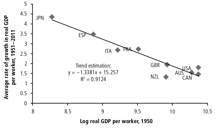
Another regularity emerging from the empirical evidence on economic growth in OECD countries is the convergence of the levels of GDP per worker over the past 60 years. In principle, within a group of countries, convergence occurs if countries with low initial levels of GDP per worker grow faster than countries with higher levels of GDP per worker. This means that the initial level of GDP per capita and the average rate of growth must be negatively related. The sample in Table 5.1 can be employed to evaluate the extent of convergence among OECD countries.

Figure 5.1 plots a scatter diagram, with the natural logarithm of GDP per worker in 1950 on the horizontal axis and the average rate of growth of real GDP per worker from 1950 to 2011 on the vertical axis. The figure also includes a linear trend fitted through the points of the scatter and the results from the least squares estimation of the fitted line. The slope of the fitted trend is negative, which is consistent with the hypothesis of convergence (i.e. that lower initial standards of living correspond to higher average growth).

The observation of the apparent convergence in the level of GDP per worker among OECD countries led several economists to believe in the hypothesis of absolute convergence, according to which relatively poor countries tend to grow faster than richer countries, and in the long run GDP per worker converges to a unique level in all countries. From a policy perspective, absolute convergence implies that poor countries will soon catch up with the standard of living of richer countries, and poverty will ultimately disappear around the world.

Stylised facts: rest of the world

Since Kaldor first published his empirical evidence on economic growth, many economists have researched whether or not, and to what extent, the stylised facts observed in the rich part of the world found any empirical support outside the OECD area.

This empirical evidence shows two fundamental results. First, over the last 60 years the standard of living has not increased in several African, Asian, and South American countries. This evidence contradicts Kaldor’s first stylised fact, as it shows that over long periods of time countries can experience zero or even negative growth. Second, the hypothesis of absolute convergence has no empirical support from a worldwide perspective.

Figure 5.2 considers economic convergence from 1960 to 2011, within a sample including seven selected Asian countries and the USA. Note that the Asian countries are mostly located towards the north-west corner of the scatter, whereas the USA is located in the south-east corner. That is, all the selected Asian countries had initial levels of GDP per worker lower than the USA, but grew at a faster pace over the chosen time period.

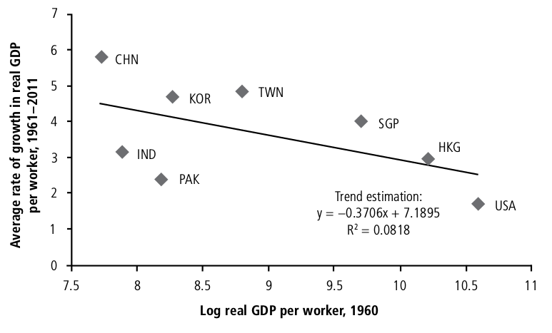
This evidence at first appears consistent with the hypothesis of absolute convergence, which is also confirmed by the estimated slope of the linear trend fitted through the points of the scatter. But note that the estimated slope of the fitted line is considerably smaller than that estimated for the selected OECD countries, whereas the R 2 suggests a far poorer fit. The implication is that the evidence for convergence beyond OECD countries does not appear particularly robust. This implies that the hypothesis of convergence may not apply to all countries of the world, as suggested by absolute convergence. At best it seems to apply only to selected sub-groups of countries, such as the OECD sub-sample.

Following this observation, economists have formulated the hypothesis of conditional convergence, which states that a country’s income per worker converges to a country-specific long-run level, determined by the structural characteristics of that country. In other words, the hypothesis of conditional convergence predicts that different groups of countries should converge towards different long-run levels of GDP per worker. For instance some countries have higher saving and investment rates than others. Savings and investments accumulate in the form of physical
capital, which is then used to increase production. As a result, we should expect countries with high levels of savings and investments to have higher GDP per worker, but then GDP per worker cannot converge to the same level for all countries. Countries that invest larger fractions of their GDP in education, which contributes to increasing the quality and the productivity of labour, should be expected to approach higher levels of GDP than those countries with lower levels of investment in human capital. A third important structural characteristic is the level of population growth. High population growth implies that the physical capital used in production must be distributed across a larger and increasing number of people. Ceteris paribus, high population growth thus tends to reduce GDP
per capita, preventing absolute convergence.

From a policy perspective, conditional convergence implies that the levels of GDP per worker towards which countries converge in the long run depend upon their structural characteristics, and are not determined by their initial levels of income. As a result, in order to raise the standard of living in less developed countries, foreign aid policies should be aimed at improving the quality of these countries’ infrastructure, their education systems and their financial systems, and at limiting their population growth. Over the last 60 years, the standard of living has not increased in several African, Asian and South American countries. This contradicts Kaldor’s first fact, as it shows that over long periods of time countries can experience zero or negative growth.

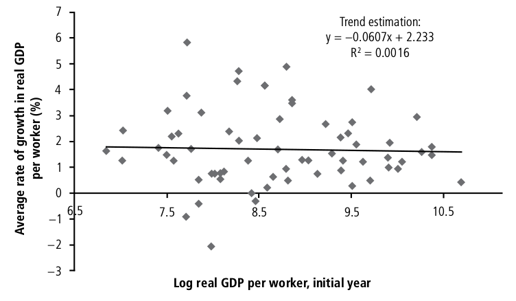
The following shows average rates of growth from a sample including all countries in Figures 5.1 and 5.2 as well as 50 additional developing countries. The scatter diagram shows little evidence of convergence from a worldwide perspective. In addition, several low-income countries have experienced per-worker growth at rates lower than high-income countries, or even negative rates. This is consistent with the hypothesis of so-called club convergence, which states that the level of GDP per worker towards which countries converge in the long run depends upon:
1. the structural characteristics of the economy
2. the initial level of income.

The second of these does not feature as part of the absolute or conditional convergence hypotheses. It implies that low income countries are destined to grow along lower growth paths, ceteris paribus. Club convergence may
imply that foreign aid policies should include income transfers from rich to poor countries, in order to allow less developed countries to reach higher growth paths. Under conditional convergence such transfers would boost
income levels in recipient countries in the short term, but would not affect their long-term growth rates.

The neoclassical production function

According to neoclassical theory, aggregate GDP (Y) is a function of the aggregate quantities of capital (K) and labour (N) used in production:

Y_t = F( K_t , N_t )

The function F(.) has the following characteristics: it is continuous, twice differentiable, exhibits constant returns to scale (CRTS), and has positive but decreasing returns to labour and capital.

The returns to scale of a production function denotes the effect on output of a given change in all productive inputs. Suppose all inputs are increased by a proportion μ. If output increases by a factor greater than μ, then the production function is said to display increasing returns to scale. If output increases by μ, then the production function is said to display CRTS. If output increases by less than μ, then the production function is said to display decreasing returns to scale. Therefore, analytically, CRTS implies that:

F(μK_t, μN_t ) = μF(K_t, N_t ) ∀ μ ≥ 0

A corollary of CRTS is that F(0) = 0. That is, an economy without capital and labour cannot produce any output.

The marginal product of a factor refers to the effect on output of a marginal increase in the quantity of a single input of production. The neoclassical production function assumes that the marginal products of capital (MPK) and labour (MPL) are positive:

MPK = ∂F(K , N )/∂K = F_K > 0
MPL = ∂F(K , N )/∂N = F_N > 0

where the symbols F_K and F_N are used to indicate the first-order derivatives of output with respect to capital and labour respectively. In addition, the increase in the marginal product occurs at a diminishing rate, that is:

F_KK < 0 , F_NN < 0

where F_KK = ∂F_K/∂K and F_NN = ∂F N/∂N

The CRTS assumption implies that the aggregate production function can be written as:

Y_t/N_t = F ((K_t/N_t),1)

which is the so-called intensive form of the production function. Setting output and capital per worker as y_t = Y_t / N_t and k_t = K_t / N_t respectively, the intensive form of the aggregate production function can be written as:

y_t = f ( k_t ), where f(k_t ) is defined as F(k_t,1).

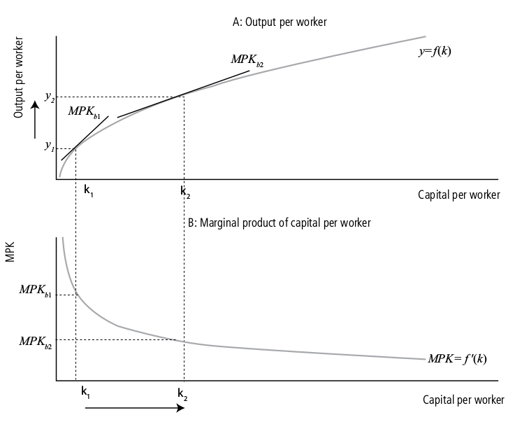
The assumption of a diminishing marginal product of capital implies that the increase in output per worker from an extra unit of capital per worker declines as the ratio K/N increases. As a result, the intensive form of the neoclassical production function inherits most properties from the aggregate production function (continuous, twice differentiable, and positive, but diminishing, returns to capital per worker). Its shape is depicted in Figure 5.4. The Figure plots output per worker as a function of capital per worker in panel A, and the marginal product of capital per worker in panel B. MPK measures the slope of the production function at every level of capital per worker. The assumption of positive but diminishing marginal products implies that the slope of the production function becomes flatter as capital increases. As a result, the MPK in panel B is a decreasing function of capital.

The Solow model: basic assumptions

The Solow model assumes that the economy consists only of households and firms operating in a competitive market. Therefore, the resource constraint of the economy is given by:

Y_t = C_t + I_t

where Y_t is total GDP, C_t is total consumption, and I_t is gross investment. Output is generated in the absence of technological progress, by a neoclassical production function:

Y_t = F(K_t,N_t )

where F is a continuous and twice differentiable function, K_t is the total stock of capital and N t is total labour. As stated in the previous section, the neoclassical production function has constant returns to scale, positive but diminishing marginal products of capital and labour, and satisfies the Inada conditions.

In a competitive market the factors of production are paid their marginal products. Therefore it follows that:

MPK = F_K = r
MPL = F_N = w

where r denotes the rental cost of capital and w measures the real wage.

Households follow a simple rule of saving a constant fraction, s, of income in every period t. As a result, aggregate consumption is a fixed fraction of output:

C_t = ( 1 − s ) Y_t = ( 1 − s ) F ( K_t , N_t )

The absence of government and the foreign sector implies that all private saving, S t , is used to finance new investment:

S_t = sY_t = sF ( K_t , N_t ) = I_t

Firms make investment both to increase the stock of capital available for production and to replace the capital lost in every period due to physical depreciation:

I_t = K_t+1 − K_t + δK_t

where K_t+1 − K_t denotes the increase in the capital stock (net investment), and δ is the rate of physical depreciation, which is assumed to be time-invariant and exogenous.

Substituting equation (5.2) into this expression and rearranging gives the dynamic equation of capital accumulation:

K_t+1 − K_t = sF(K_t , N_t ) − δK_t ,

which shows that capital changes over time because of the addition of new stock from gross investment, I_t = sF( K_t , N_t ) , and the loss of stock due to physical depreciation, δK_t

The model assumes that the size of the population in a country coincides with the labour force, and that there is no unemployment, L_t = N_t . As a result the labour force grows at the same rate as the population gN ≥ 0, and its size evolves over time according to:

N_t = (1 + g_N )N_t−1 .

Because the standard of living is measured in either per-capita or per-worker terms, it is convenient to rewrite the whole model scaling all variables by N t . We will use the small case to indicate variables measured in per-worker terms. Therefore capital, output, consumption and investment per worker are denoted, respectively, as k_t = K_t / N_t , y_t = Y_t / N_t , c_t = C_t / N_t , and i_t = I_t / N_t .

The three key equations of the basic Solow model in per-worker terms are:

Output per worker: y_t = f( k_t )
Consumption per worker: c_t = ( 1 − s ) y_t = (1 − s ) f( k_t )
Accumulation of capital per worker: k_t+1 − k_t = sf( k_t ) − ( δ + gN ) k_t .

the term sf ( k_t ) measures actual investment, whereas the term ( δ + gN ) k_t is known as break-even investment, as it measures the quantity of new investment required in each period of time in order to maintain a constant stock of capital per worker.

The Solow model: the steady state

Steady state is defined as a condition of the economy in which all endogenous variables are stable over time relative to one another. By definition, the growth rate of a ratio of two variables to one another in the steady state is zero. Such ratios in the Solow model include c_t , y_t and k_t , and their steady-state growth rates are denoted as:

g_k^* = ∆k_t^ss/k_t = 0 ; g_c^* = ∆c_t^ss/c_t = 0 ; g_y^* = ∆g_t^ss/g_t = 0

The whole dynamic in the basic Solow model is driven by the equation of capital accumulation. The dynamic of output and consumption per worker depends entirely upon the dynamic of k_t . In other words, output and consumption per worker are in steady state if and only if capital per worker is not growing.

The notion of the steady state is often associated with that of long-run equilibrium. As a result, the long-run equilibrium is defined as a condition of the economy in which all variables are constant relative to one another (i.e. in the steady state). By definition, the steady state occurs in the Solow model when k_t + 1 = k_t = k^* (i.e. the stock of capital per worker is unchanged over time). Therefore, the dynamic equation of capital accumulation (5.6) implies that a steady-state stock of capital per worker exists when actual investment equals break-even investment, sf ( k ) = ( δ + gN )k^*. Consequently, the steady-state stock of capital per worker is given by:

k^* = (s / (δ + g_N))f(k^*)

The Solow model implies that the economy follows a balanced growth path, which means that in the long run consumption, capital and output per worker all grow at the same rate (zero).

Three implications of this result are important to highlight. First, if in the steady state output and capital grow at the same rate, the steady-state capital-output ratio must be constant. Second, if the stock of capital per worker is constant in the long run, then the return on capital, MPK, must be constant in the steady state. Third, according to the basic version of the Solow model (without exogenous technical progress) consumption, output and capital per worker do not grow in the long run! This final outcome clearly contradicts the empirical evidence of permanent growth in the standard of living observed in all OECD countries and many Asian countries (Kaldor’s first stylised fact). This latter implication shows the fundamental flaw in our basic version of the Solow model, which will be
discussed further, and amended, in the next chapter.

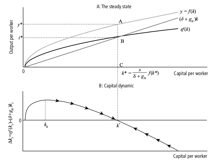
Panel A in Figure 5.5 gives a graphical representation of the basic version of the Solow model. The blue line indicates output per worker. Break-even investment is a linear function of capital per worker and, thus, represented by a straight line. Actual investment is a constant fraction of output and, thus, maintains the same concave shape of the production function. The steady state occurs when actual investment equals break-even investment, at point B. The projection of this point onto the horizontal axis gives the equilibrium stock of capital per worker, whereas the projection onto the vertical axis gives the corresponding level of investment. The projection of point B onto the production function gives the steady-state level of output per worker, indicated by point A. The segment AC measures output per worker, BC measures investment, while AB is consumption (i.e. the difference between output and actual investment).

In the Solow model there exists a unique non-zero steady-state level of capital per worker, corresponding to the value of capital per worker at which the actual investment curve coincides with the break-even line. Equation (5.6) can be employed to assess the dynamic of capital and output when the economy is not in the steady state. The basic outcome of the model is:

1. If the stock of capital per worker is lower than its steady-state value, k_t < (s / (δ + g_N) )y* , actual investment exceeds break-even investment, sf(k_t) > (δ + g_N) )_t , and the economy accumulates capital per worker, k_t+1 − k_t > 0 . When the economy accumulates capital per worker, the growth rate of capital per worker must be positive, g_k,t > 0, and GDP per worker increases over time, g_y,t > 0.

2. If the stock of capital per worker is larger than its steady-state k_t > (s / (δ + g_N) )y^*, actual investment is lower than break-even investment, sf ( k_t ) < ( δ + g_N ) k_t , and the economy is reducing its capital stock per worker over time, k_t + 1 − k_t < 0 . Thus, the growth rate of capital per worker must be negative, g k,t < 0, and, consequently, also the growth rate of GDP per worker is negative, g_y,t < 0.

Panel B of Figure 5.5 gives a graphical illustration of the dynamic behaviour of capital per worker. Whenever the actual investment curve sf(k t ) lies above the break-even investment line ( δ + g N ) k t , ∆ k t + 1 = k t + 1 − k t is positive and k t is growing over time. Conversely, when the actual investment curve sf(k t ) lies below ( δ + g N ) k t , ∆ k t + 1 is negative, and hence the stock of capital per worker, k t , is falling. The arrows on the ∆ k t + 1 line indicate this movement in k t . Note how the arrows point towards the steady state k * , indicating that k t converges towards k * for large enough values of t. Analytically, this result is written as: limk_t → ∞ kt = k* .

That is, the Solow model predicts that in the long run the economy converges towards the level of GDP per worker in equation (5.7).

To the extent that economies differ in terms of their saving rates and population growth, the predictions of the Solow model are consistent with the hypothesis of conditional convergence, since in the long run the standard of living is entirely determined by the structural characteristics of the economy. The model predicts absolute convergence under the – highly implausible – assumption that the production function f (.), the rate of saving s, the growth rate of the labour force g N , and the rate of physical depreciation δ are identical across countries. The predictions of the basic Solow model are, in general, inconsistent with the hypothesis of club convergence, since long-run growth is zero irrespective of a country’s initial level of income.

Comparative statics

Comparative statics can be carried out to evaluate short- and long-run effects of changes in the parameters of the Solow model on economic growth.

Since the long-run growth rate of GDP per worker is zero, both temporary and permanent changes in all parameters of the model can only have a temporary effect on the growth rate of GDP. However, any permanent change in a parameter of the model affects the level of GDP per worker, both in the short and in the long run.

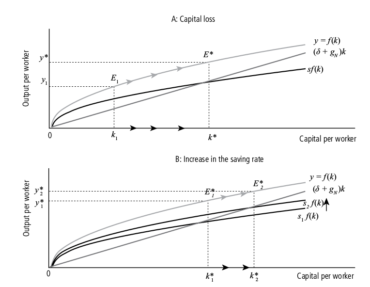
Panel A in Figure 5.6 illustrates the effect on the economy of a capital loss, which may occur for example as a result of a war that causes the destruction of part of the capital of a country. The economy is assumed to be originally in equilibrium at point E * , which corresponds to the steady-state capital stock per worker k * and the steady-state level GDP per worker y * . The capital stock suddenly drops to k 1 , and GDP per worker falls to the new level y 1 . Since at k 1 actual investment exceeds break-even investment, the economy begins to accumulate physical capital until the capital stock converges back to its equilibrium value k * . As a result of capital accumulation, the level of GDP per capita also increases and converges back to its original steady-state value y * . Therefore, the Solow model predicts that a fall in the capital stock leads to positive growth rates of capital and output per worker in the short run, but has no effect in the long run.

Panel B in Figure 5.6 illustrates the effect on the economy of an increase in the savings rate. At the initial savings rate s 1 the long-run equilibrium is at point E 1 * , which corresponds to the steady-state capital stock per worker k 1 * and the steady-state level of GDP per worker y 1 * . When the savings rate increases to s 2 > s 1 , at the initial equilibrium capital stock k 1 * actual investment exceeds break-even investment. The economy begins to accumulate capital per worker until the new steady state k 2 * is reached. Simultaneously, the increase in capital per worker increases the level of GDP per worker. Thus, the Solow model predicts that a permanent increase in the savings rate will temporarily increase the growth rate of GDP per worker, but it cannot sustain a permanent increase in the standard of living. In other words, changes in the rate of saving affect the rate of growth of GDP per worker in the short run, but not in the long run. The level of GDP per worker in the new steady state E 2 * is, though, higher than at E 1 * . Thus, the increase in saving permanently raises the level of GDP per worker.

The golden rule

We have seen so far that any change in the rate of saving alters the steady- state levels of capital, output and consumption per worker.

Since in the steady state actual investment equals break-even investment, we can regard any vertical segment between the production function curve and the break-even investment line in the Solow model as the amount of consumption attainable at a particular steady-state level of capital stock.

Therefore it is possible to define the set of possible steady-state levels of consumption per worker by taking the difference between output per worker and break-even investment per worker at any level of capital per worker (or, equivalently, any savings rate). Figure 5.7 gives a graphical illustration of the steady-state consumption per worker function, which is written analytically as:

c * = f ( k * ) − ( δ + g N ) k * .

The shape of the steady-state consumption per worker function is entirely determined by the properties of the production function and, since consumption cannot be negative, the consumption function is defined when 0 ≤ k * ≤ f ( k * ) / (δ + g N ). The figure shows that the consumption function is strictly concave and has a unique maximum. As a result, there must be a rate of saving such that (i) the economy is in steady state and (ii) households’ consumption is maximised across all possible steady-state values.

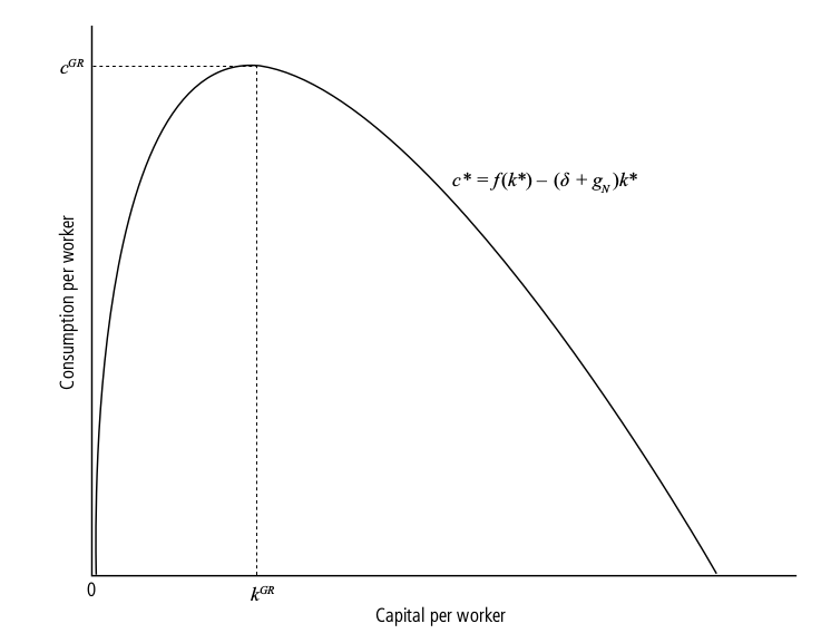
The golden rule (GR) level of capital per worker k GR is defined as the steady-state level of capital per worker that maximises consumption per worker.

Analytically, GR capital per worker is computed by choosing the k GR that maximises consumption per worker in equation c^* = f ( k^* ) − ( δ + g_N ) k^*(5.8):

This is a standard maximisation problem that is solved by setting the first- order derivative of c * with respect to k GR equal to zero: (5.9)

Equation (5.9) shows that at the GR the slope of the production function is equal to that of break-even investment, or equivalently, the marginal product of capital equals the sum of the rate of physical depreciation and the growth rate of the population.

It can be shown that the second order derivative of equation (5.9) is which confirms that k GR maximises steady-state consumption. Figure 5.8 plots in the top panel the GR level of capital per worker and shows that this coincides with the slope of the production function, f k = MPK, being equal to the slope of the break-even investment line, δ + g N . The bottom panel shows how consumption changes as the capital stock increases. When the capital stock is below its golden rule value k GR , an increase in capital also raises steady-state consumption. Vice versa, when the capital stock is larger than its GR value an increase in capital reduces steady-state consumption.

Note that to the extent that households in the economy derive utility from consumption, the GR condition yields the level of capital per worker that maximises steady-state consumer welfare. This is important because it allows evaluation of the long-run impact on consumption of changes in the savings rate. Figure 5.9 illustrates an economy that is in equilibrium at point A, where the capital stock is at the GR level, so that maximum consumption is given by the segment AB. The increase in the rate of saving to s 1 > s GR results in a sudden reduction in consumption, measured by the segment BC. In the long run the economy converges to the higher equilibrium capital stock k 1 * . The long run level of consumption per worker is given by the segment DE, which is also lower than AB.

Therefore the increase in the savings rate reduces consumption both in the short and the long run. Conversely, an economy that is in equilibrium with a stock of capital per worker larger than its GR level is said to be dynamically inefficient, because a reduction in the savings rate would increase consumption both in the short and in the long run.

Blanchard, O., Johnson, D.R., (2013) Macroeconomics (sixth edition), Pearson

Chapter 10: The Facts of Growth

The defining characteristic of a logarithmic scale is that the same proportional increase in a variable is represented by the same distance on the vertical axis.

**10-1 Measuring the Standard of Living**

Output per person is also called output per capita. And given that output and income are always equal, it is also called income per person, or income per capita.

When we focus on comparing standards of living, we get more meaningful comparisons by correcting for the two effects we just discussed—variations in exchange rates, and systematic differences in prices across countries. Such adjusted real GDP numbers, which you can think of as measures of purchasing power across time or across countries, are called purchasing power parity (PPP) numbers.

What matters for people’s welfare is their consumption rather than their income. One might therefore want to use consumption per person rather than output per person as a measure of the standard of living.

Thinking about the production side, we may be interested in differences in productivity rather than in differences in the standard of living across countries. In this case, the right measure is output per worker—or, even better, output per hour worked if the information about total hours worked is available—rather than out- put per person.

**10-2 Growth in Rich Countries since 1950**

the evolution of output per person (GDP divided by population, measured at PPP prices) for France, Japan, the United Kingdom, and the United States, since 1950.

There has been a large increase in output per person.
There has been a convergence of output per person across countries.

These numbers show what is sometimes called the force of compounding (like compound interest). Suppose we
could find a policy measure that permanently increased the growth rate by 1% per year. This would lead, after 40 years, to a standard of living 48% higher than it would have been without the policy—a substantial difference.

The second and third columns of Table 10-1 show that the levels of output per person have converged (become closer) over time: The numbers for output per person are much more similar in 2009 than they were in 1950.
This convergence of levels of output per person across countries is not specific to the four countries we are looking at. It extends to the set of OECD countries.

**10-3 A Broader Look across Time and Space**

... there is agreement among economic historians about the main evolutions over the last 2,000 years.

From the end of the Roman Empire to roughly year 1500, there was essentially no growth of output per person in Europe: Most workers were employed in agriculture in which there was little technological progress.

This period of stagnation of output per person is often called the Malthusian era.

Eventually, Europe was able to escape this trap. From about 1500 to 1700, growth of output per person turned positive, but it was still small—only around 0.1% per year. It then increased to just 0.2% per year from 1700 to 1820. Starting with the Industrial Revolution, growth rates increased, but from 1820 to 1950 the growth rate of output per person in the United States was still only 1.5% per year. On the scale of human history, therefore, sustained growth of output per person—especially the high growth rates we have seen since 1950—is definitely a recent phenomenon.

plots the average annual growth rate of output per person for the year 1960, for 76 countries... The striking feature of Figure 10-3 is that there is no clear pattern: It is not the case that, in general, countries that were behind in 1960 have grown faster. Some have, but many have clearly not.

Convergence is also visible for many Asian countries.. The picture is different, however, for African countries. Most African countries (represented by squares) were very poor in 1960, and most have not done well over the period. Many have suffered from either internal or external conflicts. Eight of them have had negative growth of output per person... between 1960 and 2009.

Growth theory takes many of the institutes of a country as given. Development economics asks what institutions are needed to sustain steady growth, and how they can be put in place.

**10-4 Thinking About Growth: A Primer**

The starting point for any theory of growth must be an aggregate production function, a specification of the relation between aggregate output and the inputs in production.

Aggregate production function: Y = F(K,N) (lol, no land)

The function F depends on the state of technology. The higher the state of technology, the higher F1K, N2 for a given K and a given N.

Increases in capital lead to smaller and smaller increases in capitalas decreasing returns to capital. There are decreasing returns to labor as well.

The production function we have written down, together with the assumption of constant returns to scale, implies that there is a simple relation between output per worker and capital per worker.

Y/N = F(K/N, N/N) = F (K.N, 1)

Note that Y>N is output per worker, K>N is capital per worker.

As capital per worker increases, so does output per worker. Note that the curve is drawn so that increases in capital lead to smaller and smaller increases in output. This follows from the property that there are decreasing returns to capital.

Increases in capital per worker: Movements along the production function.
Improvements in the state of technology: Shifts (up) of the production function.

An improvement in technology shifts the production function up, leading to an increase in output per worker for a given level of capital per worker.

Growth coming from capital accumulation and from technological progress

A higher saving rate cannot permanently increase the growth rate of output. But a higher saving rate can sustain a higher level of output.

Sustained growth requires sustained technological progress. This really follows from the previous proposition: Given that the two factors that can lead to an increase in output are capital accumulation and technological progress, if capital accumulation cannot sustain growth forever, then technological progress must be the key to growth.

Summary

* Over long periods, fluctuations in output are dwarfed by growth— the steady increase of aggregate output over time.

* Looking at growth in four rich countries (France, Japan, the United Kingdom, and the United States) since 1950, two main facts emerge:
1. All four countries have experienced strong growth and a large increase in the standard of living. Growth from 1950 to 2009 increased real output per person by a factor of 3.1 in the United States and by a factor of 10.2 in Japan.
2. The levels of output per person across the four countries have converged over time. Put another way, those countries that were behind have grown faster, reducing the gap between them and the current leader, the United States.

* Looking at the evidence across a broader set of countries and a longer period, the following facts emerge:
1. On the scale of human history, sustained output growth is a recent phenomenon.
2. The convergence of levels of output per person is not a worldwide phenomenon. Many Asian countries are
rapidly catching up, but most African countries have both low levels of output per person and low growth
rates.

* To think about growth, economists start from an aggregate production function relating aggregate output to two factors of production: capital and labor. How much output is produced given these inputs depends on the state of technology.

* Under the assumption of constant returns, the aggregate production function implies that increases in output per worker can come either from increases in capital per worker or from improvements in the state of technology.

* Capital accumulation by itself cannot permanently sustain growth of output per person. Nevertheless, how much a country saves is very important because the saving rate determines the level of output per person, if not its growth rate.

* Sustained growth of output per person is ultimately due to technological progress. Perhaps the most important question in growth theory is what the determinants of technological progress are.

Chapter 11: Saving, Capital Accumulation, and Output

Over long periods—an important qualification to which we will return—an economy’s growth rate does not depend on its saving rate. Even if the saving rate does not permanently affect the growth rate, it does affect the level of output and the standard of living. An increase in the saving rate would lead to higher growth for some time and eventually to a higher standard of living.

**11-1 Interactions between Output and Capital**

At the center of the determination of output in the long run are two relations between output and capital:

* The amount of capital determines the amount of output being produced.
* The amount of output determines the amount of saving and, in turn, the amount of capital being accumulated over time.

Output per worker (Y/N) is an increasing function of capital per worker (K/N).

Capital Stock ==> Output/Income ==> Saving/Investment ==> Change in Capital Stock ==> Capital Stock

I = S + (T - G), assume T-G = 0, I = S and is proportional income S = sY (The parameter s is the saving rate. It has a value between zero and 1), I_t = sY_t.

Investment is proportional to output: The higher output is, the higher is saving and so the higher is investment.

he evolution of the capital stock is then given by
K_t+1 = (1 - d)K_t + I_t

Divide each side by N (Number of workers). Capital per worker at the beginning of year t + 1 is equal to capital per worker at the beginning of year t, adjusted for depreciation, plus investment per worker during year t, which is equal to the saving rate times output per worker during year t.

The change in the capital stock per worker—represented by the difference between the two terms on the left—is equal to saving per worker—represented by the first term on the right—minus depreciation—represented by the second term on the right. This equation gives us the second relation between output and capital per worker.

**11-2 The Implications of Alternative Saving Rates**

* Investment per worker, the first term on the right. The level of capital per worker this year determines output per worker this year. Given the saving rate, output per worker determines the amount of saving per worker and thus the investment per worker this year.

* Depreciation per worker, the second term on the right. The capital stock per worker determines the amount of depreciation per worker this year.

When capital and output are low, investment exceeds depreciation and capital increases. When capital and output are high, investment is less than depreciation and capital decreases. (figure 11-2)

Our analysis leads to a three-part answer:
1. The saving rate has no effect on the long-run growth rate of output per worker, which is equal to zero. We have seen that, eventually, the economy converges to a constant level of output per worker. In other words, in the long run, the growth rate of output is equal to zero, no matter what the saving rate is.

Think of what would be needed to sustain a constant positive growth rate of output per worker in the long run. Capital per worker would have to increase. Not only that, but, because of decreasing returns to capital, it would have to increase faster than output per worker. This implies that each year the economy would have to save a larger and larger fraction of its output and dedicate it to capital accumulation (e.g., Soviet Union, 1950-1990)

2. Nonetheless, the saving rate determines the level of output per worker in the long run. Other things being equal, countries with a higher saving rate will achieve tion is a statement about the higher output per worker in the long run. Note that the first proposition is a statement about the growth rate of output per worker. The second proposition is a statement about the level of output per worker.

3. An increase in the saving rate will lead to higher growth of output per worker for some time, but not forever. From the first, we know that an increase in the saving rate does not affect the long-run growth rate of output per worker, which remains equal to zero. From the second, we know that an increase in the saving rate leads to an increase in the long-run level of output per worker. It follows that, as output per worker increases to its new higher level in response to the increase in the saving rate, the economy will go through a period of positive growth. This period of growth will come to an end when the economy reaches its new steady state.

An economy in which there is technological progress has a positive growth rate of output per worker, even in the long run. This long-run growth rate is independent of the saving rate—the extension of the first result just discussed. The saving rate affects the level of output per worker, however—the extension of the second result. An increase in the saving rate leads to growth greater than steady-state growth rate for some time until the economy reaches its new higher path the extension of our third result.

Recall: Saving is the sum of private plus public saving. Governments can affect the saving rate in various ways. First, they can vary public saving. Given private saving, positive public saving—a budget surplus, in other words—leads to higher overall saving. Conversely, negative public saving—a budget deficit—leads to lower overall saving. Second, governments can use taxes to affect private saving. For example, they can give tax breaks to people who save, making it more attractive to save and thus increasing private saving.

What saving rate should governments aim for? To think about the answer, we must shift our focus from the behavior of output to the behavior of consumption. The reason: What matters to people is not how much is produced, but how much they consume. An increase in saving must come initially at the expense of lower consumption. A change in the saving rate this year has no effect on capital this year, and consequently no effect on output and income this year. So an increase in saving comes initially with an equal decrease in consumption.

An economy in which the saving rate is (and has always been) zero is an economy in which capital is equal to zero. In this case, output is also equal to zero, and so is consumption. A saving rate equal to zero implies zero consumption in the long run.

Now consider an economy in which the saving rate is equal to one: People save all their income. The level of capital, and thus output, in this economy will be very high. But because people save all of their income, consumption is equal to zero. What happens is that the economy is carrying an excessive amount of capital: Simply maintaining that level of output requires that all output be devoted to replacing depreciation! A saving rate equal to one also implies zero consumption in the long run.

These two extreme cases mean that there must be some value of the saving rate between zero and one that maximizes the steady-state level of consumption. Increases in the saving rate below this value lead to a decrease in consumption initially, but to an increase in consumption in the long run. Increases in the saving rate beyond this value decrease consumption not only initially, but also in the long run.

This happens because the increase in capital associated with the increase in the saving rate leads to only a small increase in output—an increase that is too small to cover the increased depreciation: In other words, the economy carries too much capital. The level of capital associated with the value of the saving rate that yields the highest level of consumption in steady state is known as the **golden-rule level**
of capital. Increases in capital beyond the golden-rule level reduce steady-state consumption.

An increase in the saving rate leads to an increase, then to a decrease in steady-state con-
sumption per worker. There is an optional level of highest possible consumption with a mid-point of saving. What percentage is that? S_G to C/N

11-3 Getting a Sense of Magnitudes
Assume the production function is Y = sqrtK sqrtN (which means both K and N are equal). Output per worker equals the square root of capital per worker.

An increase in the saving rate leads to an increase in the steady- state level of output. But how long does it take for output to reach its new steady-state level? Put another way, by how much and for how long does an increase in the saving rate affect the growth rate?

The difference between in vestment and depreciation is greatest at the beginning. This is why capital accumulation, is why capital accumulation, highest at the beginning.

11-4 Physical versus Human Capital

We have concentrated so far on physical capital—machines, plants, office buildings, and so on. But economies have another type of capital: the set of skills of the workers in the economy, or what economists call human capital. An economy with many highly skilled workers is likely to be much more productive than an economy in which most workers cannot read or write. (It is still crap to call it 'capital')

Our conclusions about physical capital accumulation remain valid: An increase in the saving rate increases steady-state physical capital per worker and therefore increases output per worker. But our conclusions now extend to human capital accumulation as well. An increase in how much society “saves” in the form of human capital—through education and on-the-job training—increases steady-state human capital per worker, which leads to an increase in output per worker. Our extended model gives us a richer picture of how of output per worker is determined. In the long run, it tells us that output per worker depends on both how much society saves and how much it spends on education.

A country that saves more or spends more on education will achieve a higher level of output per worker in steady state. It did not say that by saving or spending more on education a country can sustain permanently higher growth of output per worker.

Models that generate steady growth even without technological progress are called models of endogenous growth to reflect the fact that in those models—in contrast to the model we saw in earlier sections of this chapter—the growth rate depends, even in the long run, on variables such as the saving rate and the rate of spending on education.

The current consensus is as follows:

* Output per worker depends on the level of both physical capital per worker and human capital per worker. Both forms of capital can be accumulated, one through physical investment, the other through education and training. Increasing either the saving rate and/or the fraction of output spent on education and training can lead to much higher levels of output per worker in the long run. However, given the rate of technological progress, such measures do not lead to a permanently higher growth rate.

* Note the qualifier in the last proposition: given the rate of technological progress. But is technological progress unrelated to the level of human capital in the economy? Can’t a better educated labor force lead to a higher rate of technological progress? These questions take us to the topic of the next chapter, the sources and the effects of technological progress.

Summary
-------

* In the long run, the evolution of output is determined by two relations. (To make the reading of this summary easier, we shall omit “per worker” in what follows.) First, the level of output depends on the amount of capital. Second, capital accumulation depends on the level of output, which determines saving and investment.

* These interactions between capital and output imply that, starting from any level of capital (and ignoring technological progress, the topic of Chapter 12), an economy converges in the long run to a steady-state (constant) level of capital. Associated with this level of capital is a steady-state level of output.

* The steady-state level of capital, and thus the steady-state level of output, depends positively on the saving rate. A higher saving rate leads to a higher steady-state level of output; during the transition to the new steady state, a higher saving rate leads to positive output growth. But (again ignoring technological progress) in the long run, the growth rate of output is equal to zero and so does not depend on the saving rate.

* An increase in the saving rate requires an initial decrease in consumption. In the long run, the increase in the saving rate may lead to an increase or a decrease in consumption, depending on whether the economy is below or above the golden-rule level of capital, the level of capital at which steady-state consumption is highest.

* Most countries have a level of capital below the golden-rule level. Thus, an increase in the saving rate leads to an initial decrease in consumption followed by an increase in consumption in the long run. When considering whether or not to adopt policy measures aimed at changing a country’s saving rate, policy makers must decide how much weight to put on the welfare of current generations versus the welfare of future generations.

* While most of the analysis of this chapter focuses on the effects of physical capital accumulation, output depends on the levels of both physical and human capital. Both forms of capital can be accumulated, one through investment, the other through education and training. Increasing the saving rate and/or the fraction of output spent on education and training can lead to large increases in output in the long run.

Dornbusch, R., S. Fischer and R. Startz Macroeconomics (2011)

Chapter 3: Growth and Accumulation

• Economic growth is due to growth in inputs, such as labor and capital, and to improvements in technology.
• Capital accumulates through saving and investment.
• The long-run level of output per person depends positively on the saving rate and negatively on the rate of population growth.
• The neoclassical growth model suggests that the standard of living in poor countries will eventually converge to the level in wealthy countries.

The production function provides a quantitative link between inputs and outputs. As a simplification, we first assume that labor ( N ) and capital ( K ) are the only important inputs. Equation (1) shows that output ( Y ) depends on inputs and the level of technology ( A ). (We say that A represents the level of technology because the higher A is, the more output is produced for a given level of inputs. Sometimes A is just called “productivity,” a more neutral term than “technology.”)

Y = AF (K, N )

More input means more output. In other words, the marginal product of labor, or MPL (the increase in output generated by increased labor), and the marginal product of capital, or MPK (the increase in output generated by increased capital), are both positive.

delta Y = [ (1 - theta) * delta N/N] + (theta + deltaK/K) + deltaA/A

i.e., output growth = (labour share) * labour growth + capital share * capital growth + technology growth

(theta = .25 makes the Cobb-Douglas function a very good approximation to the real economy, so the Cobb-Douglas function can be written as Y = AK .25 N .75)

* Labor and capital each contribute an amount equal to their individual growth rates multiplied by the share of that input in income .
* The rate of improvement of technology, called technical progress, or the growth of total factor productivity, is the third term in equation

The growth rate of total factor productivity is the amount by which output would increase as a result of improvements in methods of production, with all inputs unchanged.

Solow Residual, concentrates on A

deltaA/A = delta Y/Y - [ (1 - theta) * delta N/N] - (theta + deltaK/K)

Adding human capital, H , we can write the production function as Y = AF(K, H, N ). An influential article by Mankiw, Romer, and Weil suggests that the production function is consistent with factor shares of one-third each for physical capital, raw labor, and human capital.

Neoclassical growth theory begins with a simplifying assumption. We start our analysis by pretending that there is no technological progress. This implies that the economy reaches a long-run level of output and capital called the steady-state equilibrium . The steady-state equilibrium for the economy is the combination of per capita GDP and per capita capital where the economy will remain at rest, that is, where per capita economic variables are no longer changing, delta y = 0 and delat k = 0.

The investment required to maintain a given level, k , of capital per capita depends on population growth and the depreciation rate, the rate at which machines wear out. The investment required to maintain a constant level of capital per capita is ( n + d ) k .

The net change in capital per capita, delta k , is the excess of saving over required investment.

At that steady state, both k and y are constant. With per capita income constant, aggregate income is growing at the same rate as population, that is, at rate n . It follows that the steady-state growth rate is not affected by the saving rate. This is one of the key results of neoclassical growth theory.

In the short run, an increase in the saving rate raises the growth rate of output. In the long run, an increase in the saving rate will lead to an increase in the level of capital and output per head, and will leave the growth rate of output unchanged.

* An increase in the rate of population growth reduces the steady-state level of capital per head, k , and output per head, y .
* An increase in the rate of population growth increases the steady-state rate of growth of aggregate output.

Summary
-------
1. Neoclassical growth theory accounts for growth in output as a function of growth in inputs, particularly capital and labor. The relative importance of each input depends on its factor share.
2. Labor is the most important input.
3. Long-run growth results from improvements in technology.
4. Absent technological improvement, output per person will eventually converge to a steady-state value. Steady-state output per person depends positively on the saving rate and negatively on the rate of population growth.
5. The long-run rate of growth does not depend on the saving rate.

Mankiw, N. G. Macroeconomics. (Worth, 2009)

Chapter 7 Economic Growth I: Capital Accumulation and Population Growth

The supply of goods in the Solow model is based on the production function, which states that output depends on the capital stock and the labor force:
Y = F(K, L).

Designate quantities per worker with lowercase letters, so y = Y/L is output per worker, and k = K/L is capital per worker. We can then write the production function as
y = f (k),

The slope of this production function shows how much extra output a worker produces when given an extra unit of capital. This amount is the marginal product of capital MPK. Mathematically, we write
MPK = f(k + 1) − f (k).

The Demand for Goods and the Consumption Function The demand for goods in the Solow model comes from consumption and investment. In other words, output per worker y is divided between consumption per worker c and investment per worker i:
y = c + i.

The Solow model assumes that each year people save a fraction s of their income and consume a fraction (1 – s). We can express this idea with the following consumption function, where s, the saving rate, is a number between zero and one.

c = (1 − s)y,

To see what this consumption function implies for investment, substitute (1 – s)y for c in the national income accounts identity:
y = (1 − s)y + i.

Rearrange the terms to obtain
i = sy.

Two forces influence the capital stock: investment and depreciation. Investment is expenditure on new plant and equipment, and it causes the capital stock to rise. Depreciation is the wearing out of old capital, and it causes the capital stock to fall.

Where delta k is the change in the capital stock between one year and the next. Because investment i equals sf(k), we can write this as delta k = sf(k) − deprec (lc delta) k.

We therefore call k* the steady-state level of capital.

Investment, Depreciation, and the Steady State The steady-state level of capital k* is the level at which investment equals depreciation, indicating
that the amount of capital will not change over time. Below k* investment exceeds depreciation, so the capital stock grows. Above k* investment is less than depreciation, so the capital stock shrinks. (figure 7-4). The steady state represents the long-run equilibrium of the economy.

If the saving rate is high, the economy will have a large capital stock and a high level of output in the steady state. If the saving rate is low, the economy will have a small capital stock and a low level of output in the steady state. The long-run consequences of a reduced saving rate are a lower capital stock and lower national income. This is why many economists are critical of persistent budget deficits.

Policies that alter the steady-state growth rate of income per person are said to have a growth effect; we will see examples of such policies in the next chapter. By contrast, a higher saving rate is said to have a level effect, because only the level of income per person—not its growth rate—is influenced by the saving rate in the steady state.

How can we tell whether an economy is at the Golden Rule level? To answer this question, we must first determine steady-state consumption per worker. Then we can see which steady state provides the most consumption. To find steady-state consumption per worker, we begin with the national income accounts identity
y = c + i
and rearrange it as
c = y – i.

Steady-state output per worker is f(k*), where k* is the steady-state capital stock per worker. Furthermore, because the capital stock is not changing in the steady state, investment equals depreciation k*. Substituting f(k*) for y and lcdelta k* for i, we can write steady-state consumption per worker as

c* = f (k*) − lcdeltak*.

According to this equation, steady-state consumption is what’s left of steady-state output after paying for steady-state depreciation. This equation shows that an increase in steady-state capital has two opposing effects on steady-state consumption. On the one hand, more capital means more output. On the other hand, more capital also means that more output must be used to replace capital that is wearing out.

Steady-state consumption is the gap between output and depreciation. This figure shows that there is one level of the capital stock—the Golden Rule level k* gold —that maximizes consumption.

Reducing Saving When Starting With More Capital Than in the Golden Rule Steady State This figure shows what happens over time to output, consumption, and investment when the economy begins with more capital than the Golden Rule level and the saving rate is reduced. The reduction in the saving rate (at time t 0 ) causes an immediate increase in consumption and an equal decrease in investment. Over time, as the cap- ital stock falls, output, consumption, and investment fall together. Because the economy began with too much capital, the new steady state has a higher level of consumption than the initial steady state.

Increasing Saving When Starting With Less Capital Than in the Golden Rule Steady State This figure shows what happens over time to output, consumption, and investment when the economy begins with less capital than the Golden Rule level and the saving rate is increased. The increase in the saving rate (at time t 0 ) causes an immediate drop in consumption and an equal jump in investment. Over time, as the capital stock grows, output, consumption, and investment increase together. Because the economy began with less capital than the Golden Rule level, the new steady state has a higher level of consumption than the initial steady state.

Population Growth in the Solow Model Depreciation and population growth are two reasons the capital stock per worker shrinks. If n is the rate of population growth and is the d ( + rate of depreciation, then d n)k is break-even investment—the amount of investment necessary to keep constant the capital stock per worker k. For the economy to be in a steady state, investment sf(k) must offset the effects of depreciation and population growth ( + n)k. This is d crossing of represented by the the two curves.

The Impact of Population Growth An increase in the rate of population growth from n 1 to n 2 shifts the line representing population growth and depreciation upward. The new steady state k * 2 has a lower level of capital per worker than the initial steady state k *1 . Thus, the Solow model predicts that economies with higher rates of population growth will have lower levels of capital per worker and therefore lower incomes.

Summary
-------

Summary

1. The Solow growth model shows that in the long run, an economy’s rate of saving determines the size of its capital stock and thus its level of production. The higher the rate of saving, the higher the stock of capital and the higher the level of output.

2. In the Solow model, an increase in the rate of saving has a level effect on income per person: it causes a period of rapid growth, but eventually that growth slows as the new steady state is reached. Thus, although a high saving rate yields a high steady-state level of output, saving by itself cannot generate persistent economic growth.

3. The level of capital that maximizes steady-state consumption is called the Golden Rule level. If an economy has more capital than in the Golden Rule steady state, then reducing saving will increase consumption at all points in time. By contrast, if the economy has less capital than in the Golden Rule steady state, then reaching the Golden Rule requires increased investment and thus lower consumption for current generations.

4. The Solow model shows that an economy’s rate of population growth is another long-run determinant of the standard of living. According to the Solow model, the higher the rate of population growth, the lower the steady-state levels of capital per worker and output per worker. Other theories highlight other effects of population growth. Malthus suggested that population growth will strain the natural resources necessary to produce food; Kremer suggested that a large population may promote technological progress.