Aims of the chapter

This chapter surveys the Mundell–Fleming model for the analysis of monetary and fiscal policy in an open economy. The first part of the chapter revises the balance of payments line under alternative assumptions about international capital mobility. The second part of the chapter introduces the Mundell–Fleming model, which treats the exchange rate as an endogenous variable rather than a policy instrument. We revise the policy prescriptions of the Mundell–Fleming model under perfect capital mobility and without capital mobility, and then focus on the description of
the model under imperfect capital mobility.

By the end of this chapter, and having completed the Essential reading and activities, you should be able to:
• state the determinants of the BP line, and explain how its slope changes under alternative assumptions about international capital mobility
• recall the policy prescriptions of the Mundell–Fleming model under
perfect capital mobility and with no capital mobility
• describe the macroeconomic policy prescriptions of the Mundell–Fleming model under imperfect capital mobility
• discuss the medium-run adjustment mechanism in an open economy under alternative exchange rate regimes
• discuss the determinants and implications of an exchange rate crisis.

This chapter is mainly centred on the assessment of the Mundell–Fleming model, which analyses the simultaneous determination of output, the interest rate and the exchange rate in an open economy. The Mundell–Fleming model extends the IS–LM framework to an open economy, by combining the IS–LM curves with a balance of payments (BP) line. For this reason it is also referred to as the IS–LM–BP model. Note that the three main textbooks describe the Mundell–Fleming model only under the assumption of perfect capital mobility. Descriptions of the model under the other two assumptions about capital mobility are usually provided in international macroeconomics textbooks.

It is important to note that under the assumption of perfect capital mobility the analytical and graphical description of the Mundell–Fleming model varies between the three main textbooks, even though the policy predictions are almost entirely unchanged. The model reduces to three equations: the IS curve, the LM curve and the BP line. It assumes that the expected exchange rate responds immediately and one-for-one to changes in the current exchange rate. Under these assumptions, the model predicts that fiscal policy is a very effective tool of macroeconomic stabilisation under fixed exchange rates, but it is completely ineffective under flexible exchange rates because the increase in output resulting from a fiscal expansion is entirely crowded out by a reduction in net exports resulting from exchange rate appreciation. Conversely, the canonical Mundell–Fleming model predicts that monetary policy is an ineffective stabilisation tool under fixed exchange rates, but it is very effective under flexible exchange rates.

If you are using Blanchard and Johnson, the treatment of the Mundell–Fleming model is slightly different from the canonical model, as the BP equation is replaced with the UIP condition, and the expected exchange rate is assumed to be fixed and responding less than one-for-one to movements in the current exchange rate. In these circumstances, an appreciation of the current exchange rate implies an expected future depreciation, allowing higher nominal interest rates to be sustained. The policy prescriptions of the revised model under fixed exchange rates are the same as those arising from the canonical version. However, they differ under flexible exchange rates in that fiscal policy is still an effective stabilisation tool, since the exchange rate appreciation resulting from a fiscal expansion will only partially crowd out the corresponding increase in output.

The next sections provide a summary of the material. We begin by revising the determinants of the BP line and discussing how its slope varies according to the degree of capital mobility in international financial markets. Next, we revise the main policy prescriptions of the Mundell–Fleming model under perfect capital mobility and with no capital mobility. The chapter then gives a great emphasis to describing the Mundell–Fleming model under imperfect capital mobility, and explaining its implications for fiscal and monetary policy in the short run. Finally, we look at exchange rate crises by highlighting the factors that may lead to such a crisis, as well as its economic and policy implications.

The balance of payments (BP ) curve and capital mobility

In an open economy, external balance occurs when the BP equilibrium condition in equation (7.1) of the previous chapter is satisfied, that is:
BP = NX + CA = 0,

where NX indicates the net trade position and CA the capital account. The components of this equilibrium condition depend, in turn, on the real exchange rate, the international interest rate differential and the level of domestic income.

BP = NX ( ε,Y ) + CA ( i − i * ) = 0, (8.1)

where ε is the real exchange rate, Y is domestic income and i and i measure the domestic and foreign interest rates respectively. Equation (8.1) shows that the real exchange rate affects the trade (current account) balance, as it determines the price of domestic goods relative to foreign goods, whereas the interest rate differential ultimately drives the flow of capital to and from a country. The level of domestic income matters in determining total imports, as we saw in the previous chapter. Equation (8.1) defines the so called BP curve, which plots the combinations of domestic interest rates and domestic income levels for which the balance of payments is in equilibrium (i.e. there is external balance), for a given
level of the real exchange rate. It is useful to distinguish three situations where the balance of payments is in equilibrium:

1. Both the current and capital accounts are in balance.
2. A current account surplus is just compensated by a capital account deficit.
3. A current account deficit is just counterbalanced by a capital account surplus.

In general, for a given value of ε the slope of the BP curve is determined by two key variables. First, the **marginal propensity to import**, which determines how the current account balance responds to an increase in domestic income. Second the **degree of capital mobility**, which determines the sensitivity of capital flows to interest differentials. Under **perfect capital mobility**, the composition of the balance of payments is entirely determined by the capital account. Any change, however small, in the domestic interest rate relative to the world interest rate causes massive capital flows, far more than is required to finance a trade deficit or offset a surplus. Thus, no positive or negative interest rate differential can be sustained in equilibrium: the BP curve is horizontal in income–interest rate space, and intercepts the vertical axis at a point where i=i * .

Conversely, under no capital mobility, CA = 0, and the composition of the balance of payments is entirely determined by the current account. The BP line is vertical in income–interest rate space, since for any given ε there is a unique level of income such that imports balance exports. The intermediate case is one of imperfect capital mobility. Here the BP line is positively sloped in income–interest rate space, since an increase in income, which worsens the current account, may be offset by an increase in the domestic interest rate, which attracts a finite amount of additional foreign capital.

The Mundell–Fleming model with perfect and no capital mobility

The standard Mundell–Fleming model predicts that in the short run under perfect capital mobility and a fixed exchange rate:
1. monetary policy is entirely ineffective in increasing output
2. fiscal policy is extremely effective in increasing output.

It contrast, the canonical Mundell–Fleming model predicts that in the short run under perfect capital mobility and a flexible exchange rate:
1. monetary policy is extremely effective in increasing output
2. fiscal policy is ineffective in increasing output.

Note that Blanchard and Johnson propose a version of the Mundell–Fleming model slightly modified from the canonical one presented in Dornbusch et al. and Mankiw. To understand the difference between the two versions of the model, recall that the canonical Mundell–Fleming model assumes that the expected exchange rate responds immediately and one-for-one to movements in the current exchange rate, that is E t = E t e + 1 . Under this assumption, the BP curve is analytically represented by equality between the domestic and world interest rates. Instead, Blanchard and Johnson’s version of the model assumes that the expected exchange rate is fixed, in the sense that it responds less than one-for-one to movements in the current exchange rate. As a result, the current exchange rate can be different from the expected exchange rate, E t ≠ E t e + 1 . In this instance, the BP curve is replaced by the more generic UIP condition:

Et = absE^et+1 (1+i/1+i^*)

which states that interest rate differentials can persist in equilibrium, provided they are compensated for by expected currency movements. In the special case that the expected exchange rate responds immediately and one-for-one to movements in the current exchange rate, E t = E t e + 1 , the UIP condition reduces to the BP curve employed by the canonical Mundell–Fleming model under perfect capital mobility. Otherwise UIP predicts that if the domestic currency is expected to depreciate, E t > E t e + 1 , then the domestic interest rate must exceed the foreign interest rate. In this case, foreign investors are still indifferent between domestic and foreign bonds, since the expected capital loss from holding domestic bonds is compensated by the higher interest rate. Vice versa, if the domestic currency is expected to appreciate, E t < E t + 1 , the domestic interest rate must be lower than the foreign interest rate. In this case, financial investors will still purchase domestic bonds since they expect to be compensated by a future capital gain.

The key result is that investors will still hold low interest rate bonds because they expect to be compensated by a future appreciation of the exchange rate. In other words, even under perfect capital mobility, interest rate differentials may not cause massive inflows and outflows of capital, as assumed in the canonical model.

This alternative version of the Mundell–Fleming model yields almost the same predictions as the canonical one, the only exception being for fiscal policy, which becomes somewhat effective under flexible exchange rates and perfect capital mobility.

Under a fixed exchange rate and if there is no capital mobility, so that BP is a vertical line, both expansionary fiscal and monetary policies are completely ineffective in increasing output. This is because all expansions raise imports, and thus yield balance of payments deficits, which require reductions in the money supply to bring output back down. In contrast, both expansionary fiscal and monetary policies are very effective in increasing output under a flexible exchange rate if there is no capital mobility, since balance of payments deficits induce a currency depreciation that raises net exports and allows a higher level of income to persist in equilibrium.

The Mundell–Fleming model under imperfect capital mobility and a fixed exchange rate

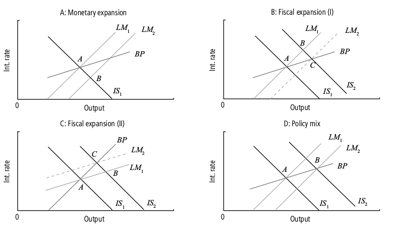
Figure 8.1 displays the effects of monetary and fiscal policy in an open economy under imperfect capital mobility with a fixed exchange rate. In each panel of the diagram the initial equilibrium is at point A, where BP = 0. Panel A shows that a monetary expansion causes a rightward shift in the LM curve, from LM 1 to LM 2 . As a result, the new short-run equilibrium is at point B, corresponding to a balance of payments deficit and a higher level of output. The balance of payments is in deficit because the increase in the money supply raises output, which leads to higher imports and a current account deficit, and reduces the interest rate, causing a capital account deficit. Panels B and C show the effect of a fiscal expansion. In general, a fiscal expansion increases both output and the interest rate.

The rise in income generates a current account deficit, while the increase in the interest rate leads to a capital account surplus. The net effect on the balance of payments depends on the relative slopes of the LM and BP curves. If the LM curve is steeper than the BP curve, as in Panel B, then the balance of payments is in surplus (point B). If the LM curve is flatter than the BP curve, as in panel C, then the balance of payments is in deficit (point B). Thus, the relative sensitivity of international capital flows and income sensitivity of imports – together with the income sensitivity of money demand (which determines the slope of the curve) – are the crucial factors in determining whether an expansionary fiscal policy leads to an external deficit or surplus. Finally, Panel D shows how a mix of monetary and fiscal policy can be employed to increase output without inducing a balance of payments deficit or surplus (simultaneous fiscal and monetary expansion).

An important issue is that balance of payments surpluses and deficits are not sustainable on their own. A balance of payments surplus corresponds to an excess supply of foreign currency, which must be bought by the domestic central bank. The central bank pays for its purchase of foreign currency with domestic currency. Thus, a balance of payments surplus increases the money supply of the economy because the central bank must purchase foreign exchange. Similarly, a balance of payments deficit implies there is an excess demand for foreign currency, which must be provided by the domestic central bank. The central bank withdraws domestic currency from circulation when it sells its foreign currency. Thus, a balance of payments deficit decreases the money supply of the economy because the central bank must sell foreign exchange.

From a graphical point of view, this implies that after a monetary expansion (see Panel A, Figure 8.1), the balance of payments deficit causes a monetary contraction that gradually shifts the LM curve back to its original position, LM. The final position of the economy after a fiscal expansion depends on the position of the LM curve relative to the BP line. If the LM curve is steeper than the BP curve, as in Panel B, then the BP surplus triggers a monetary expansion which further increases output. The new equilibrium is at point C on the BP line. If the LM curve is flatter than the BP curve, as in Panel C, then the BP deficit causes a monetary contraction which partially offsets the initial increase in income. In this case the new equilibrium is at point C on the BP line.

Central banks may, however, be able to sustain monetary expansions under fixed exchange rates by conducting so-called sterilisation policies. These policies work by changing the relative supply of short-term and long-term assets available domestically, in such a way that investors are willing to accept a lower short-term interest rate to hold any given quantity of short-term assets. This is equivalent to engineering a downward shift in the BP line in panel A, so that equilibrium might be restored close to point B.But most economists are sceptical about the extent to which sterilisation policy can be successful in practice. While it may allow limited monetary expansions to be sustained under a fixed exchange rate, ultimately monetary policy must be devoted largely to sustaining the currency peg.

To sum up, the Mundell–Fleming model predicts that with a fixed exchange rate regime under imperfect capital mobility and with no sterilisation policy:
1. monetary policy is entirely ineffective in increasing output
2. fiscal policy is extremely effective in increasing output

The Mundell–Fleming model under imperfect capital mobility and a flexible exchange rate

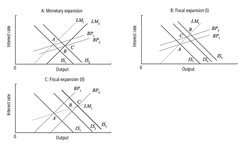
The analysis of monetary and fiscal policy in an open economy with imperfect capital mobility changes considerably under a flexible exchange rate. Recall that under a flexible exchange rate balance of payments surpluses or deficits do not automatically require rises and falls in the money supply. This is because balance of payments surpluses and deficits result in rises and falls in the real exchange rate, and thus movements in the BP and IS curves rather than the LM curve. In particular, if the real exchange rate rises then the trade balance deteriorates for any level of income. Consequently, both the BP curve and the IS curve shift leftwards. Conversely, a fall in the real exchange rate improves the net trade position. This leads to a rightward shift of both the BP curve and the IS curve. Figure 8.2 displays the effects of monetary and fiscal policy under imperfect capital mobility and with a flexible exchange rate. In each panel of the diagram the initial equilibrium is at point A, where BP 1 = 0. Panel A considers a monetary expansion which shifts the LM curve rightward, from LM 1 to LM 2 , hence leading to a balance of payments deficit at point B. At B, there is excess demand for foreign currency and excess supply of domestic currency on the foreign exchange market. Under a flexible exchange rate regime, this implies that the real exchange rate will fall, shifting BP rightwards to BP 2 and the IS curve rightwards to IS 2 . The
new equilibrium is at point C, at a higher output level. Thus, under a flexible exchange rate regime (and unlike a fixed exchange rate regime), monetary policy is very effective in increasing output.

In contrast, the effectiveness of fiscal policy under a flexible exchange-rate regime and imperfect capital mobility is more ambiguous. Panel B in Figure 8.2 shows the case of an LM curve steeper than the BP line. The economy begins at point A. A fiscal policy expansion implies a rightwards shift of the IS curve to IS 2 , so the economy moves to point B. However, at point B the balance of payments is in surplus, and thus there will be a rise in the exchange rate which, in turn, shifts BP upwards to BP 2 and IS backwards from IS 2 to IS 3 . The final equilibrium is achieved at point C. Consequently, with imperfect capital mobility and an LM curve steeper than the BP line, a fiscal expansion is less powerful under a flexible exchange rate regime than under a fixed exchange rate regime. The above conclusion is reversed if the LM curve is flatter than the BP line, as illustrated in Panel C of Figure 8.2. In this case, a fiscal expansion leads to a balance of payments deficit and consequently a fall in the exchange rate. The reduction in the exchange rate shifts rightwards both the IS and BP curves, until the internal and external equilibrium is reached at point C. Therefore, with imperfect capital mobility and an LM curve flatter than the BP line, a fiscal expansion is more powerful under a flexible exchange-rate regime than under a fixed exchange rate regime.

Exchange rate crisis

If an economy with a fixed exchange rate is experiencing a recession or the central parity is too high, the domestic central bank could be tempted either to devaluate the exchange rate or even to switch to a floating exchange rate system to accelerate the speed of recovery. An exchange rate crisis occurs when financial market investors believe that the domestic central bank is likely to devalue the exchange rate in the near future.

The UIP condition implies that in order to keep the central parity the domestic central bank has to increase the interest rate by an amount equal to the expected devaluation. This may be an unfeasible policy, since a monetary contraction would further aggravate the economic recession.

The fear of an imminent devaluation or abandoning of the fixed exchange rate may trigger a so-called speculative attack, consisting of massive sales of domestic bonds for foreign bonds, resulting in a large capital outflow. In turn, this entails a large sale of domestic currency for foreign currency, which is needed by financial investors to purchase safer foreign bonds. Without the intervention of the central bank in the domestic foreign exchange market, the large demand for foreign currency would lead to a depreciation of the exchange rate. However, the intervention of the domestic central bank in the foreign exchange market would cause a large and unsustainable fall in its foreign currency reserves.

As a result, to stop the speculative attack the first option for the central bank is to try to convince the financial market about its commitment to the existing parity – for instance through TV announcements or press conferences. If this is not sufficient, the domestic central bank may increase the interest rate, though probably by an amount lower than that required under the UIP condition. If the speculative attack continues, the central bank may be forced to either devalue, or to abandon the fixed exchange rate regime entirely.

The key insight here is that the fear of an imminent devaluation, even when this is groundless, can trigger an exchange rate crisis that leads to the breakdown of a fixed exchange rate arrangement. It is important that you relate this analysis to the 1973 breakdown of the Bretton Woods agreement, the 1992 European Monetary System crisis, and the Asian crisis at the end of the 1990s.

Blanchard, O., Johnson, D.R., (2013) Macroeconomics (sixth edition), Pearson

Chapter 20: Output, The Interest Rate and The Exchange Rate

We examine the implications of equilibrium in both the goods market and financial markets, including the foreign exchange market. This allows us to characterize the joint movements of output, the interest rate, and the exchange rate in an open economy.

Chapter 21: Exchange Rate Regimes

Equilibrium in the goods market was the focus of Chapter 19, where we derived the equilibrium condition (equation (19.4)):

Y = C(Y - T ) + I (Y, r ) + G - IM (Y, e) / P + X (Y *, P)

For the goods market to be in equilibrium, output (the left side of the equation) must be equal to the demand for domestic goods (the right side of the equation). The demand for domestic goods is equal to consumption, C, plus investment, I, plus gov-
ernment spending, G, minus the value of imports, IM/e, plus exports, X.

Goods market equilibrium (IS): Output = Demand for domestic goods.

We shall assume, throughout the chapter, that the Marshall-Lerner condition holds. Under this condition, an increase in the real exchange rate—a real appreciation—leads to a decrease in net exports

For our purposes, the main implication of equation (20.1) is that both the real in-terest rate and the real exchange rate affect demand, and in turn equilibrium output:

* An increase in the real interest rate leads to a decrease in investment spending, and, as a result, to a decrease in the demand for domestic goods. This leads, through the multiplier, to a decrease in output.
* An increase in the real exchange rate leads to a shift in demand toward foreign goods, and, as a result, to a decrease in net exports. The decrease in net exports decreases the demand for domestic goods. This leads, through the multiplier, to a
decrease in output.

* A decrease in the nominal exchange rate—a nominal depreciation—leads, one-for-one, to a decrease in the real exchange rate—a real depreciation. Conversely, an increase in the nominal exchange rate—a nominal appreciation—leads, one-for-one, to an increase in the real exchange rate—a real appreciation.

20-2 Equilibrium in Financial Markets

When we looked at the determination of the interest rate in the IS–LM model in Chapter 5, we wrote the condition that the supply of money be equal to the demand for money as
M/P = YL(i)

In an open economy, the demand for domestic money is still mostly a demand by domestic residents, so this doesn't change much.

Financial investors, domestic or foreign, go for the highest expected rate of return. This implies that, in equilibrium, both do- mestic bonds and foreign bonds must have the same expected rate of return; other-wise, investors would be willing to hold only one or the other, but not both, and this could not be an equilibrium.

* An increase in the domestic interest rate leads to an increase in the exchange rate.
* An increase in the foreign interest rate leads to a decrease in the exchange rate.
* An increase in the expected future exchange rate leads to an increase in the current exchange rate.

The Relation between the Interest Rate and the Exchange Rate Implied by Interest Parity
A higher domestic interest rate leads to a higher exchange rate—an appreciation.

20-3 Putting Goods and Financial Markets Together

Goods-market equilibrium implies that output depends, among other factors, on the interest rate and the exchange rate:

Y = C(Y - T) + I(Y, i ) + G + NX (Y, Y *, E)

The interest rate in turn is determined by the equality of money supply and money demand:

M/P = YL (i)

And the interest parity condition implies a negative relation between the domestic interest rate and the exchange rate:

E = (1 + i) / (1 + i*) - barE^e

Together, these three relations determine output, the interest rate, and the exchange rate.

* The first effect, which was already present in a closed economy, is the direct effect on investment: A higher interest rate leads to a decrease in investment, a decrease in the demand for domestic goods, and a decrease in output.
* The second effect, which is only present in the open economy, is the effect through the exchange rate: An increase in the domestic interest rate leads to an increase in the exchange rate—an appreciation. The appreciation, which makes domestic goods more expensive relative to foreign goods, leads to a decrease in net exports, and therefore to a decrease in the demand for domestic goods and a decrease in output.

The IS–LM Model in the Open Economy
An increase in the interest rate reduces output both directly and indirectly (through the exchange rate): The IS curve is downward sloping. Given the real money stock, an increase in output increases the interest rate: The LM curve is upward sloping.

20-4 The Effects of Policy in an Open Economy

The Effects of an Increase in Government Spending
An increase in government spending leads to an increase in output, an increase in the interest rate, and an appreciation. An increase in government spending shifts the IS curve to the right. It shifts neither the LM curve nor the interest parity line.

A monetary contraction leads to a decrease in output, an increase in the interest rate, and an appreciation.

20-5 Fixed Exchange Rates

A decrease in the exchange rate under a regime of fixed exchange rates is called a devaluation rather than a depreciation, and an increase in the exchange rate under a regime of fixed exchange is called a revaluation rather than an appreciation.

Pegging or no pegging, the exchange rate and the nominal interest rate must satisfy the interest parity condition. Now suppose the country pegs the exchange rate at E, so the current exchange rate E t = E. If financial and foreign exchange markets believe that the exchange rate will remain pegged at this value, then their expectation of the future exchange rate, E t e + 1 , is also equal to E. If financial investors expect the exchange rate to remain unchanged, they will require the same nominal interest rate in both countries. Under a fixed exchange rate and perfect capital mobility, the domestic interest rate must be equal to the foreign interest rate.

Under flexible exchange rates, a fiscal expansion increases output from Y A to Y B . Under fixed exchange rates, output increases from Y A to Y C . p437

Under fixed exchange rates fiscal policy is more powerful than it is under flexible exchange rates. This is because fiscal policy triggers monetary accommodation.

As this chapter comes to an end, a question should have started to form in your mind: Why would a country choose to fix its exchange rate? You have seen a number of reasons why this appears to be a bad idea:
* By fixing the exchange rate, a country gives up a powerful tool for correcting trade imbalances or changing the level of economic activity.
* By committing to a particular exchange rate, a country also gives up control of its interest rate. Not only that, but the country must match movements in the foreign interest rate, at the risk of unwanted effects on its own activity.
* Although the country retains control of fiscal policy, one policy instrument may not be enough. As you saw in Chapter 19, for example, a fiscal expansion can help the economy get out of a recession, but only at the cost of a larger trade deficit. And a country that wants, for example, to decrease its budget deficit cannot, under fixed exchange rates, use monetary policy to offset the contractionary effect of its fiscal policy on output.

* In an open economy, the demand for domestic goods depends both on the interest rate and on the exchange rate. An increase in the interest rate decreases the demand for domestic goods. An increase in the exchange rate—an appreciation—also decreases the demand for domestic goods.

* The interest rate is determined by the equality of money demand and money supply. The exchange rate is determined by the interest parity condition, which states that domestic and foreign bonds must have the same expected rate of return in terms of domestic currency.

* Given the expected future exchange rate and the foreign interest rate, increases in the domestic interest rate lead to an increase in the exchange rate—an appreciation. Decreases in the domestic interest rate lead to a decrease in the exchange rate—a depreciation.

* Under flexible exchange rates, an expansionary fiscal policy leads to an increase in output, an increase in the interest rate, and an appreciation.

* Under flexible exchange rates, a contractionary monetary policy leads to a decrease in output, an increase in the interest rate, and an appreciation.

* There are many types of exchange rate arrangements. They range from fully flexible exchange rates to crawling pegs, to fixed exchange rates (or pegs), to the adoption of a common currency. Under fixed exchange rates, a country maintains a fixed exchange rate in terms of a foreign currency or a basket of currencies.

* Under fixed exchange rates and the interest parity condition, a country must maintain an interest rate equal to the foreign interest rate. The central bank loses the use of monetary policy as a policy instrument. Fiscal policy becomes more powerful than under flexible exchange rates, however, because fiscal policy triggers monetary accommodation, and so does not lead to offsetting changes in the domestic interest rate and exchange rate.

Mankiw, N. G. Macroeconomics. (Worth, 2009)

Chapter 12: The Open Economy Revisited: The Mundell–Fleming Model and the Exchange-Rate Regime

The Mundell–Fleming model makes one important and extreme assumption: it assumes that the economy being studied is a small open economy with perfect capital mobility. That is, the economy can borrow or lend as much as it wants in world financial markets and, as a result, the economy’s interest rate is determined by the world interest rate.

12-1 The Mundell–Fleming Model

Mathematically, we can write this assumption as r = r*.

This world interest rate is assumed to be exogenously fixed because the economy is sufficiently small relative to the world economy that it can borrow or lend as much as it wants in world financial markets without affecting the world interest rate.

The LM* Curve Panel (a) shows the standard LM curve [which graphs the equation M/P = L(r, Y)] together with a horizontal line representing the world interest rate r *. The intersection of these two curves determines the level of income, regardless of the exchange rate. Therefore, as panel (b) shows, the LM* curve is vertical.

Mundell–Fleming model plots the goods-market equilibrium condition IS* and the money market equilibrium condition LM*. Both curves are drawn holding the interest rate constant at the world interest rate. The intersection of these two curves shows the level of income and the exchange rate that satisfy equilibrium both in the goods market and in the money market.

12-2 The Small Open Economy Under Floating Exchange Rates

A Fiscal Expansion Under Floating Exchange Rates. An increase in government purchases or a decrease in taxes shifts the IS* curve to the right. This raises the exchange rate but has no effect on income.

A Monetary Expansion Under Floating Exchange Rates An increase in the money supply shifts the LM* curve to the right, lowering the exchange rate and raising income.

A Trade Restriction Under Floating Exchange Rates
A tariff or an import quota shifts the net-exports schedule in panel (a) to the right. As a result, the IS* curve in panel (b) shifts to the right, raising the exchange rate and leaving income unchanged.

12-3 The Small Open Economy Under Fixed Exchange Rates

How a Fixed Exchange Rate Governs the Money Supply In panel (a), the equilibrium exchange rate initially exceeds the fixed level. Arbitrageurs will buy foreign currency in foreign-exchange markets and sell it to the Fed for a profit. This process automatically increases the money supply, shifting the LM* curve to the right and lowering the exchange rate. In panel (b), the equilibrium exchange rate is initially below the fixed level. Arbitrageurs will buy dollars in foreign-exchange markets and use them to buy foreign currency from the Fed. This process automatically reduces the money supply, shifting the LM* curve to the left and raising the exchange rate.

A Fiscal Expansion Under Fixed Exchange Rates
A fiscal expansion shifts the IS* curve to the right. To maintain the fixed exchange rate, the Fed must increase the money supply, thereby shifting the LM* curve to the right. Hence, in contrast to the case of floating exchange rates, under fixed exchange rates a fiscal expansion raises income.

A Monetary Expansion Under Fixed Exchange Rates If the Fed tries to increase the money supply—for example, by buying bonds from the public—it will put downward pressure on the exchange rate. To maintain the fixed exchange rate, the money supply and the LM* curve must return to their initial positions. Hence, under fixed exchange rates, normal monetary policy is ineffectual.

A country with a fixed exchange rate can, however, conduct a type of monetary policy: it can decide to change the level at which the exchange rate is fixed. A reduction in the official value of the currency is called a devaluation, and an increase in its official value is called a revaluation. In the Mundell–Fleming model, a devaluation shifts the LM* curve to the right; it acts like an increase in the money supply under a floating exchange rate. A devaluation thus expands net exports and raises aggregate income. Conversely, a revaluation shifts the LM* curve to the left, reduces net exports, and lowers aggregate income.

A Trade Restriction Under Fixed Exchange Rates. A tariff or an import quota shifts the IS* curve to the right. This induces an increase in the money supply to maintain the fixed exchange rate. Hence, aggregate income increases.

				
				Floating			Fixed
			Y	e	NX		Y	e	NX
Fiscal Expansion	0	Up	Down		Up	0	0		
Monetary Expansion	Up	Down	Up		0	0	0
Import Restriction	0	Up	0		Up	0	Up

12-4 Interest Rate Differentials

So far, our analysis has assumed that the interest rate in a small open economy is equal to the world interest rate: r = r*. To some extent, however, interest rates differ around the world. We now extend our analysis by considering the causes and effects of international interest rate differentials.

To incorporate interest rate differentials into the Mundell–Fleming model, we assume that the interest rate in our small open economy is determined by the world interest rate plus a risk premium : theta. r = r* + theta

An Increase in the Risk Premium. An increase in the risk premium associated with a country drives up its interest rate. Because the higher interest rate reduces investment, the IS* curve shifts to the left. Because it also reduces money demand, the LM* curve shifts to the right. Income rises, and the currency depreciates.

12-5 Should Exchange Rates Be Floating or Fixed?

The primary argument for a floating exchange rate is that it allows monetary policy to be used for other purposes. Under fixed rates, monetary policy is committed to the single goal of maintaining the exchange rate at its announced level.

The introduction of a common currency has its costs. The most important is that the nations of Europe are no longer able to conduct their own monetary policies. Instead, the European Central Bank, with the participation of all member countries, sets a single monetary policy for all of Europe. When a recession hits one country but not others in Europe, that country does not have the tool of monetary policy to combat the downturn.

Why, according to the euro critics, is monetary union a bad idea for Europe if it works so well in the United States? These economists argue that the United States is different from Europe in two important ways. First, labor is more mobile among U.S. states than among European countries. This is in part because the United States has a common language and in part because most Americans are descended from immigrants, who have shown a willingness to move. Therefore, when a regional recession occurs, U.S. workers are more likely to move from high-unemployment states to low-unemployment states. Second, the United States has a strong central government that can use fiscal policy—such as the federal income tax—to redistribute resources among regions. Because Europe does not have these two advantages, it bears a larger cost when it restricts itself to a single monetary policy.

The analysis of exchange-rate regimes leads to a simple conclusion: you can’t have it all. To be more precise, it is impossible for a nation to have free capital flows, a fixed exchange rate, and independent monetary policy. This fact, often called the impossible trinity.

12-6 From the Short Run to the Long Run: The Mundell–Fleming Model With a Changing Price Level

Mundell–Fleming as a Theory of Aggregate Demand Panel (a) shows that when the price level falls, the LM* curve shifts to the right. The equilibrium level of income rises. Panel (b) shows that this negative relationship between P and Y is summarized by the aggregate demand curve.

The Short-Run and Long-Run Equilibria in a Small Open Economy Point K in both pan- els shows the equilibrium under the Keynesian assumption that the price level is fixed at P 1 . Point C in both panels shows the equilibrium under the classical assumption that the price level adjusts to maintain income at its natural level Y − .

12-7 A Concluding Reminder

1. The Mundell–Fleming model is the IS–LM model for a small open economy. It takes the price level as given and then shows what causes fluctuations in income and the exchange rate.

2. The Mundell–Fleming model shows that fiscal policy does not influence aggregate income under floating exchange rates. A fiscal expansion causes the currency to appreciate, reducing net exports and offsetting the usual expansionary impact on aggregate income. Fiscal policy does influence aggregate income under fixed exchange rates.

3. The Mundell–Fleming model shows that monetary policy does not influence aggregate income under fixed exchange rates. Any attempt to expand the money supply is futile, because the money supply must adjust to ensure that the exchange rate stays at its announced level. Monetary policy does influence aggregate income under floating exchange rates.

4. If investors are wary of holding assets in a country, the interest rate in that country may exceed the world interest rate by some risk premium. According to the Mundell–Fleming model, an increase in the risk premium causes the interest rate to rise and the currency of that country to depreciate.

5. There are advantages to both floating and fixed exchange rates. Floating exchange rates leave monetary policymakers free to pursue objectives other than exchange-rate stability. Fixed exchange rates reduce some of the uncertainty in international business transactions. When deciding on an exchange-rate regime, policymakers are constrained by the fact that it is impossible for a nation to have free capital flows, a fixed exchange rate, and independent monetary policy.