Aims of the chapter

This chapter revises microfounded theories of consumption, with particular attention given to the life cycle, permanent income, and random walk theories. We discuss the motivation behind each of these theories, illustrate their main policy implications, and compare their predictions with those arising from Keynesian consumption theory. The chapter also illustrates the Ricardian equivalence proposition and highlights the interplay between forward-looking behaviour, rational expectations and macroeconomic policy effectiveness.

• explain the implications of the Keynesian consumption function and the essence of the consumption puzzle
• define the basic analytical framework underpinning the microfounded approach to aggregate consumption
• describe the life cycle, permanent income and random walk hypotheses and critically assess the extent of their policy implications
• discuss the relevance and policy prescriptions of the Ricardian equivalence proposition.

This chapter discusses the motivations underpinning four key theories of consumption. We start with the **Keynesian theory of consumption**
which takes a macroeconomic perspective and assumes aggregate consumption to be a function of aggregate disposable income. This theory has three fundamental shortcomings:

1. it is a static theory of aggregate consumption
2. some of its predictions are difficult to reconcile with the empirical evidence (consumption puzzle)
3. it is based on the implausible assumption that aggregate consumption depends exclusively upon current aggregate income

We contrast the Keynesian theory with the predictions of three modern theories of consumption: the life cycle hypothesis (LCH) of Franco Modigliani, the permanent income hypothesis (PIH) of Milton Friedman and the random walk hypothesis (RWH) of Robert Hall. These three consumption theories reflect a new approach to macroeconomics, since each of them derives aggregate demand for consumption from an assessment of the optimal behaviour of each consumer living in the economy, under the assumption that economic agents are forward-looking and have rational expectations.

As well as providing a more realistic and consistent description of aggregate consumption, the new theories also have several implications for the role and the effectiveness of macroeconomic policy, which are substantially different from those arising from the standard Keynesian framework. First, modern consumption theories show that the effect of a tax cut on aggregate consumption depends on whether this measure is perceived as a temporary or a permanent policy, since rational and forward-looking consumers tend to save, rather than consume, any temporary increase in income. A related implication is that of the Ricardian equivalence proposition, which shows that – under the joint assumptions of perfect capital markets, an absence of uncertainty and an infinite lifetime horizon – no government can stimulate private consumption by cutting taxes and financing the resulting deficit with a bond issue. This is because rational and forward-looking consumers anticipate that the government will increase taxes in the future in order to repay the outstanding debt and, therefore, will save the income arising from the tax cut in order to repay debt in the future.

The Keynesian consumption function, and beyond

The Keynesian consumption function (KCF), which we have already encountered in Chapter 2, assumes that aggregate consumption depends on current disposable income, and is unaffected by changes in the interest rate. Analytically, the KCF can be written as:

C_t = c_0 + c_1 YD_t , (9.1)

where C t indicates aggregate consumption in period t, the term YD t = Y t – T t measures disposable income in period t as the difference between income and taxes in that period, and the parameters c 0 and c 1 indicate a constant term and the marginal propensity to consume respectively. The KCF yields at least two important predictions about aggregate consumption:

1. The average propensity to consume (APC), as measured by the consumption–output ratio, should decline as income increases over long periods of time.
2. Changes in aggregate consumption are entirely driven by changes in current aggregate income, irrespective of whether the change in income is temporary or permanent.

There are two major problems with the KCF. First, the empirical evidence arising from long-term time series data on the consumption–output ratio is inconsistent with the first prediction.

Cross-sectional analyses, which look at the distribution of consumption and income among all individuals living in a country over a short period of time, originally supported the view of a declining APC predicted by the KCF.

In contrast, the analysis of long-term time series data showed the APC to be roughly constant over very long periods of time. This contradicting evidence gave rise to the so-called consumption puzzle. As a result of this puzzle economists began to believe in the existence of two consumption functions: a short-term consumption function, observed in cross-sectional data or short-term time series, which is characterised by a falling APC; and a long-term consumption function, which is observed in long-term time series data and is characterised by a constant APC.

The second prediction of the KCF was questioned by several economists, on the ground that it is implausible to assume that people do not take into account their future income when making their consumption plans, and that permanent and temporary changes in income have the same effect on consumption.

In the rest of the chapter we will revise three theories of consumption which attempted to address these issues:
• the life cycle hypothesis (LCH)
• the permanent income hypothesis (PIH) and
• the random walk hypothesis (RWH).

The three models have two common characteristics. First, they are microfounded theories of consumption, in the sense that they first assess the optimal consumption choice of each individual in the economy, and then determine aggregate consumption as the outcome of the optimal choice of all individuals collectively. In the basic version of each model consumers are all assumed to be identical, so that the analysis can proceed as if there were just a single consumer in the economy (a representative consumer or Robinson Crusoe economy).

Second, each model assumes that consumers are forward-looking and plan consumption over the entire course of their lives. Consequently, current consumption depends upon lifetime wealth, rather than current income alone. Wealth is defined as the sum of non-human and human wealth. Non-human wealth includes real assets (houses, cars, machineries) and financial assets (bank deposits, bonds, stocks). Individuals can have either positive or negative non-human wealth. In the former case they are savers or lenders, in the latter they are borrowers. Human wealth instead
refers to the present value of after-tax labour income that each individual expects to earn over the course of their life. The standard assumption in these models is that each individual in the economy may have some non-human wealth at the beginning of their life, but by the end of their life they cannot leave any outstanding debt or bequest. This implies that the present value of each individual’s consumption must be equal to their total wealth, W 0 . Assuming that each individual lives only for two periods, their budget constraint is written as:

c t + (1 / (1 + r) ) c t + 1 = a 0 + y t + a 0 + y t + ( 1 / (1 + r) ) y t + 1 = W 0 (9.2)

where r denotes the interest rate, a 0 the initial level of non-human
wealth, y t + 1/1+r and c t + (1/1+r) cr1
y t + 1 the present value of current and future income,
c t + 1 is the present value of current and future consumption.
The constraint in equation (9.2) is also referred to as the intertemporal budget constraint (IBC).

The Fisher model of intertemporal consumption

We now revise the basic Fisher model of the optimal consumption allocation for a representative consumer who lives for two periods – the present period and a future period – indicated, respectively, by t and t+1. Consumption in each period is denoted by c t and c t+1 , and the consumer’s utility function is described by:

U = u ( c t ) + (1 / (1 + ρ) u ( c t + 1 ) , (9.3)

where u(c t ) is the utility from consumption in the present period, u(c t+1 ) is

the consumer’s subjective discount factor, with ρ being the consumer’s subjective discount rate, meaning that the consumer is indifferent between one unit of utility in period t and (1 + ρ) units in period t +1. Under standard assumptions the instantaneous utility function u(.) is continuous and twice differentiable. In addition, the marginal utility from extra consumption is positive, u ' ( c t ) > 0 , but diminishing, u ' ' ( c t ) < 0 . This implies that indifference curves in c t – c t +1 space are convex to the origin, with their slope given by the marginal rate of substitution (MRS):

MRS = − (1+ ρ)(u ' ( c t )/u ' ( c t + 1 )),

The consumer is endowed with income levels y t and y t+1 in the two periods, and has access to a perfect capital market in which they can borrow and lend unlimited amounts at the constant interest rate r. We assume for simplicity that non-human wealth, a o , is equal to zero.

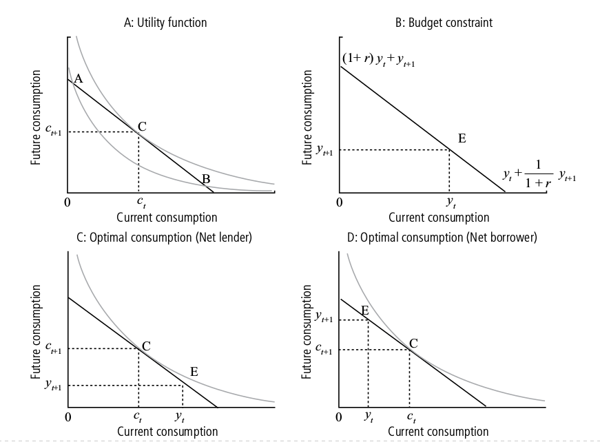
The objective of the consumer is to choose the optimal level of consumption in both periods in order to maximise their intertemporal utility function in (9.3), given the budget constraint in equation (9.2). Figure 9.1 gives a graphical illustration of the model. Panel A plots the indifference curves and the IBC. The optimal solution is at point C, namely on the highest indifference curve attainable given the budget constraint.

The panel also shows that at the optimum the consumer prefers to smooth consumption over the two periods, since point C is preferred to both point A, which gives higher future consumption relative to current consumption, and point B, which yields relatively higher current consumption. Instead, point C yields a more balanced consumption between the two periods. This result is known as consumption smoothing.

Panel B focuses on the properties of the IBC in equation (9.2). The IBC intersects the vertical axis when c t = 0, which would imply maximum consumption in period t+1, given by c t+1 = (1 + r)y t + y t+1 . Conversely, the IBC intersects the horizontal axis when c t+1 = 0, which gives the point of y t + 1 . The slope of the maximum possible current consumption, c t = y t + 1 + r

IBC is equal to –(1 + r), which represents the price of current consumption relative to future consumption: a unit reduction of consumption in the current period increases consumption by 1 + r units in the future period. Moreover, the IBC must pass through the individual income endowment, indicated by E, since it is always feasible for the individual to consume their endowment in every period.

Panel C illustrates a case in which the individual’s endowment is high in the current period and low in the future period. The optimal consumption choice implies that the individual is a lender in the current period, since c t < y t . Conversely, Panel D depicts the case of an individual who is a borrower in the current period, since c t > y t .

Analytically, the condition for an optimal consumption allocation is satisfied when the MRS equals the slope of the budget constraint or:

(1 + ρ) = (u ' ( c t ))/(u ' ( c t + 1 )) = = 1 + r . (9.4)

The above expression is known as the Euler equation, which shows that the optimal level of consumption depends upon the market interest rate, the subjective discount factor and the properties of the utility function. The left-hand side of the Euler equation is the marginal rate of substitution between current and future consumption, which measures the slope of the indifference curves of the individual at the given allocation. The right-hand side is the market price of a unit of c t in terms of c t+1 .

Consumption, interest rates and income

The two-period model of optimal consumption choice can be employed to assess the implications of changes in the interest rate and income on both the welfare and optimal consumption/saving decisions of the representative consumer. A detailed comparative statics analysis is out of the scope of this unit. However it is important that you have a clear understanding of some basic results. Here is a short summary.

Recall that an increase in the interest rate rotates the IBC around the initial endowment, making the budget line steeper. The substitution effect implies that an interest rate increase induces people to reduce current consumption, as it makes saving more attractive.

The income effect describes the consumer’s response to a change in the interest rate due to the variation of higher interest income, or payments, that it implies. As a result, it depends upon the initial borrowing or lending position of the representative consumer. If a consumer is a borrower in the current period, then an increase in the interest rate means that they have to pay more interest on any outstanding debt. If the consumer remains a borrower in the current period, then current consumption falls through the income effect when the interest rate rises. If a person is a lender, then an increase in the interest rate means that they earn more interest on their savings and the income effect is positive following a rise in the interest rate.

Overall, the response of current consumption to an increase in the interest rate is, in principle, ambiguous. The substitution effect predicts that current consumption responds negatively to the interest rate; the income effect depends on whether individuals are net borrowers or lenders. At the aggregate level, most economists believe that the negative effects dominate, and that total consumption falls when the real interest rate
rises.

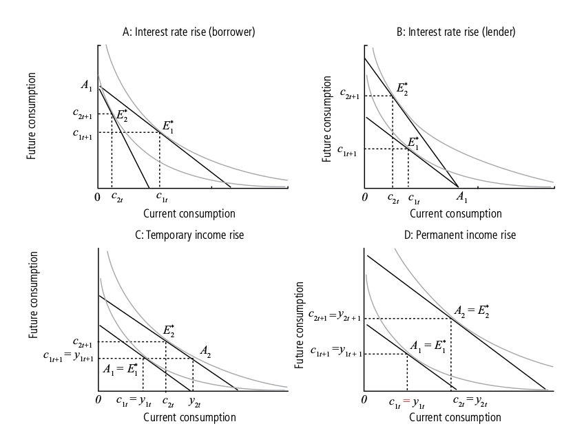
Panels A and B in Figure 9.2 illustrate two possible cases. Panel A considers the case of a consumer with no income in the first period of their life, who is therefore a borrower. An interest rate rise reduces the consumption set of the agent, and thus their welfare. It also reduces current consumption relative to future consumption as the consumer borrows less when the interest rate increases. Panel B considers the case of a consumer who is a lender, since they have no income in the future period. An interest rate rise expands the consumption set of the consumer,
increasing their welfare. It also reduces current consumption as the lender prefers to save more. In this case the income effect on current consumption is dominated by the substitution effect.

Comparative statics can also be employed to assess the likely response of consumption to changes in income. In this case it is important to distinguish between temporary and permanent increases in income. Panel C in Figure 9.2 considers a consumer whose initial endowment A 1 yields equal income in each period y 1t = y 1t+1 . The individual is also assumed to consume their endowment in each period, and the optimal consumption allocation is denoted with E * 1 . A temporary increase in current income, in the sense that the current period income rises to y 2t > y 1t while y 1t+1 is unaffected, expands the consumption set of the consumer, as the endowment shifts from A 1 to A 2 and increases both current and future consumption. As a result, a temporary increase in current income raises current consumption less than one-for-one, c 2t < y 2t . In other words, consumers save part of the temporary increase in income in order to finance higher future consumption. Panel D illustrates the effect for the same consumer of a permanent increase in income, namely an equal increase in both current income, y 2t > y 1t , and future income, y 2t+1 > y 1t+1 . The graph shows that the optimal consumption point shifts from E * 1 to E * 2 ; hence the permanent increase in income raises current (and future) consumption one-for-one, c 2t = y 2t and c 2t+1 = y 2t+1 .

The life cycle hypothesis (LCH)

The KCF assumes that individuals make consumption and saving decisions solely based upon their current income. In contrast, the LCH assumes that individuals plan their consumption and saving decisions with the objective of distributing consumption in the best possible way over the entire course of their lifetime. The central result of the model is that individuals prefer to maintain a smooth level of consumption in the face of income changes occurring over their lifetime.

The basic version of the LCH is described by assuming that the representative consumer lives for two periods. In the first period, the consumer works and earns an income w t . Part of this income is consumed, c t , and the rest, s t , is saved in the capital market at the constant interest rate r. In the second period the consumer is old and retires. They do not work, and can only finance their consumption, c t+1 , by spending the income saved when they were of working age, together with the interest accrued on that income, s t (1 + r). The intertemporal utility function is equal to that of equation (9.3), whereas the IBC is now given by:

c t + ( 1 / (1 +r ) ) ct+1 = (w - s)+ ( 1 / (1 +r) ) st (1 + r) = wt

In other words, the value of lifetime consumption equals the value of income earned when of working age. Consumption when of working age equals income minus savings. Consumption during old age equals the amount of income saved plus the interest accrued on it.

At the optimum:

u ' ( c t ) / u ' ( c t + 1 ) = (1 + r) / (1 + ρ)

which is the same Euler equation that we derived for the solution to the optimal intertemporal consumption allocation problem.

In other words, the optimal consumption choice depends again upon the value of the market interest rate relative to the individual rate of time preference, and the properties of the utility function. If r = ρ, then the consumer saves during the first period of their life an amount of income such that they can maintain a constant level of consumption throughout their lifetime. If ρ > r then the consumer prefers to consume more while they are of working age, whereas if ρ < r then they prefer to consume more after retirement.

This simplified two-period version of the model captures the fundamental essence of the LCH. Individuals prefer to smooth consumption over the entire course of their lives; hence they save in the early stages of their life when their income is high, in order to finance consumption in the late stages when their income is low. More elaborate versions of the model divide the lifetime horizon of the consumer into three stages: young, middle and old. Income is low at the young age and in old age, whereas income is high in middle age. Consumption smoothing implies that individuals borrow at the beginning of their lives, pay back their debt and save during the middle stage, and dissave towards the end of their lives. Therefore a consumer’s wealth changes over time: it increases until retirement age, and then falls to zero by the end the consumer’s lifetime.

The LCH shows that consumption depends upon wealth, and is, therefore, affected by changes in future income and the interest rate, as well as current income. In addition, the LCH explains the consumption puzzle by assuming that in cross-sectional analysis high-income consumers, those in their middle age, are likely to be above their average (lifetime) income, whereas low income people – young and old – are likely to be below their average income. As a consequence the APC falls with income. In contrast, when observed in a long-term time series the APC remains constant over time, since both current and average incomes rise over time.

The permanent income hypothesis

To illustrate the implications of the PIH we will again employ the two- period model developed so far, and assume that r = ρ. Consequently, the consumer maximises their intertemporal utility by maintaining a constant consumption level over their lifetime:

c t = c t +1 = c

Substitution of this result into the IBC yields:

c + ( c / (1 + r ) ) = yt + ( 1 / 1 + r) y t+1 (9.5)

Since consumption is constant over time, it can be factored out on the left- hand side of equation (9.5) to obtain:

c ( 1 + ( 1 / (1 + r) ) ) = = yt + ( 1 / 1 + r) y t+1 (9.6)

Equation (9.6) is the so-called consumption function, which expresses current consumption – or more generally consumption in any period t – as a function of lifetime wealth. This result is ultimately a restatement of the LCH. However, under the PIH the right-hand side in equation (9.6) is interpreted as the permanent income of the consumer, namely the amount of income that, if earned constantly every period, would allow the consumer to enjoy the same constant consumption level c. According to the PIH only permanent changes in income can affect consumption, whereas temporary changes in income have little effect, as they mainly affect saving. To illustrate this point analytically, consider again the consumption function in equation (9.6).

The response of consumption to a unit increase in income in period t is obtained by multiplying the term
(1 + r / 2 + r) by 1. The response of consumption to a unit increase in income in period t+1 is obtained by multiplying the term (1 + r ) / (2 + r) by 1 / (1 + r) which gives: (1 / 2 + r) . These are the short-term response coefficients or marginal propensities to consume from current and future income respectively, as they measure the change in consumption following a temporary increase in income. If r = 0.05, then

(1 + r )/ (2 + r) = (1 + 0.05) / (2 + 0.05) ≅ 0.5122 and 1 / ( 2 + r) = 1 / 2.05 = ≅ 0.4878

so around half of an increase in current income is saved rather than consumed. Therefore according to the PIH a temporary increase in income raises savings as well as consumption, though future income increases may also now affect current consumption (in contrast with the basic KCF).

In contrast, consider a permanent increase in income, namely a one-unit increase in income occurring at all dates. The effect on consumption is obtained by summing up all the short-run response coefficients:

(1 + r) / (2 + r) + (1 / (2 + r) ) = 1

Therefore, according to the PIH, current consumption increases one-for one as a result of a permanent increase in income.

As in the LCH, the PIH assumes that consumption depends upon wealth rather than current income alone. However, the PIH emphasises that current consumption responds much more to variations in current income if these are permanent. The PIH explains the consumption puzzle by arguing that in cross-section data high-income households have a positive temporary or transitory income, so their APC is low, whereas low-income households have only temporarily low income, so their APC is high. In long-term time series data, income rises are instead permanent, as a result of economic growth, and the temporary effects average out across consumers. For this reason consumption changes one-for-one with income, so that the APC remains constant over time.

The Ricardian equivalence proposition

An important policy implication arising from the PIH is the Ricardian Equivalence proposition, which states that the government cannot stimulate private consumption by cutting taxes and financing the resulting deficit by issuing bonds. In other words, tax cuts financed by government borrowing do not make forward-looking individuals richer. This is because tax cuts financed by issues of bonds increase public debt. Forward-looking consumers know that, some time in the future, the government has to pay back its debt, and this can only be done by increasing future taxes by an amount equal to the initial tax cut plus the interest accrued over time on that debt. For this reason, the initial increase in wealth following the tax cut is entirely offset by the future increase in taxes, and has no effect on aggregate consumption.

This point can be illustrated analytically by the following example. Suppose that r = ρ and income is taxed in every period with a lump-sum tax τ. Under these assumptions, the PIH suggests that current consumption is a function of the present value of after-tax income, which is given by:

c t = (1 + r) / (2 + r) [ y t − τ + (1 / (1 + r) ) ( y t+1 - τ ]

Suppose that the government reduces taxes in period t by the amount –∆τ and finances the resulting deficit by issuing bonds (increases borrowing) by an equal amount. In the next period, the government increases taxes by the amount ( 1 + r ) ∆ τ in order to pay the outstanding debt and the interest accrued on that debt from period t to period t +1. The impact of this policy on current consumption shows that the bond-financed tax cut does not affect lifetime wealth or consumption, since after-tax income increases in period t by ∆τ and falls in period t+1 by the same amount,

( 1 + r ) ∆ τ / (1 + r) = ∆ τ

As a result, a temporary decrease in taxation has no effect on consumption. Forward-looking consumers anticipate an offsetting future increase in taxation and save (rather than consume) the entire extra disposable income arising from the lower taxes, in order to pay for higher taxes in the future.

Dornbusch, R., S. Fischer and R. Startz Macroeconomics (2011)

Chapter 13: Consumption and Saving

• Consumption is a large but relatively stable fraction of GDP.
• Modern theories of consumption behavior link lifetime consumption to lifetime income. These theories suggest that the marginal propensity to
consume out of transitory income should be small.
• Empirical evidence suggests that both modern theories and simple Keynesian “psychological rule-of-thumb” models contribute to explaining consumption.
• The saving rate in the United States is lower than the saving rate in many other countries.

Changes in per capita disposable income and changes in per capita consumption are closely related, although the latter is less volatile than the former. Consumption does not respond much to positive or negative income spikes (short-term swings in income).

Consumption is almost perfectly predicted by consumption the previous period plus an allowance for growth.

There is a close relation, in practice, between consumption spending and disposable income. Consumption rises on average by 96 cents for each additional dollar of disposable income.

Modern consumption theory emphasizes lifetime decision making. Originally, the life- cycle hypothesis emphasized choices about how to maintain a stable standard of living in the face of changes in income over the course of life, while permanent income theory focused on forecasting the level of income available to a consumer over a lifetime. Today, these two theories have largely merged.

The life-cycle hypothesis views individuals, instead, as planning their consumption and savings behavior over long periods with the intention of allocating their consumption in the best possible way over their entire lifetimes.

Consumption is constant throughout lifetime. During the working life, lasting WL years, the individual saves, accumulating assets. At the end of the working life, the individual begins to live off these assets, dissaving for the remaining years (NL - WL) of life such that assets equal exactly zero at the end of life.

The MPC out of permanent income is large and the MPC out of transitory income is small, fairly close to zero.

Permanent income is the steady rate of expenditure a person could maintain for the rest of his or her life, given the present level of wealth and the income earned now and in the future.

A liquidity constraint exists when a consumer cannot borrow to sustain current consumption in the expectation of higher future income.

The life-cycle hypothesis is that people save largely to finance retirement. However, additional savings goals also matter. The evidence on bequests suggests that some saving is done to provide inheritances for children. There is also a growing amount of evidence to support the view that some saving is precautionary, undertaken to guard against rainy days. In other words, savings are used as a buffer stock , added to when times are good in order to maintain consumption when times are bad.

The issue raised by this argument is sometimes posed as the question, “Are government bonds net wealth?” The question goes back at least to the classical English economist David Ricardo. Renewed by Robert Barro, 23 it is known as the Barro-Ricardo equivalence proposition, or Ricardian equivalence . The proposition is that debt financing by bond issue merely postpones taxation and therefore, in many instances, is line is the budget line C later [1 r 0 ]( Y now C now ) for interest rate r 0 . The gold budget line, C later [1 r 1 ]( Y now C now ), shows that at a higher interest rate, r 1 > r 0 , you get a better return in terms of deferred consumptio for each dollar saved now.

SUMMARY
1. The life-cycle–permanent-income hypothesis (LC-PIH) predicts that the marginal propensity to consume out of permanent income is large and that the marginal propensity to consume out of transitory income is very small. Modern theories of consumption assume that individuals want to maintain relatively smooth consumption profiles over their lifetimes. Their consumption behavior is geared to their long- term consumption opportunities—permanent income or lifetime income plus wealth. With such a view, current income is only one of the determinants of consumption spending. Wealth and expected income play a role too.

2. Observed consumption is much smoother than the simple Keynesian consumption function predicts. Current consumption can be very accurately predicted from last period’s consumption. Both these observations accord well with the LC-PIH.

3. The LC-PIH is a very attractive theory, but it does not give a complete explanation of consumption behavior. Empirical evidence shows that the traditional consumption function appears to also play a role.

4. The life-cycle hypothesis suggests that the propensities of an individual to consume out of disposable income and out of wealth depend on the person’s age. It implies that saving is high (low) when income is high (low) relative to lifetime average income. It also suggests that aggregate saving depends on the growth rate of the economy and on such variables as the age distribution of the population.

5. The rate of consumption, and thus of saving, could in principle be affected by the interest rate. But the evidence, for the most part, shows little effect of interest rates on saving.

6. The Barro-Ricardo equivalence proposition notes that debt represents future taxes. It asserts that debt-financed tax cuts will not have any effect on consumption or aggregate demand.

7. The U.S. saving rate is very low by international standards. Most private saving in the United States is done by the business sector.

Mankiw, N. G. Macroeconomics. (Worth, 2009)

Chapter 17 Consumption

In previous chapters we explained consumption with a function that relates consumption to disposable income: C = C(Y − T ). This approximation allowed us to develop simple models for long-run and short-run analysis, but it is too simple to provide a complete explanation of consumer behavior.

17-1 John Maynard Keynes and the Consumption Function

The Keynesian consumption function is often written as

C = barC + cY, barC >= 0, 0 < c < 1

where C is consumption, Y is disposable income, barC is a constant, and c is the marginal propensity to consume.

On the basis of the Keynesian consumption function, these economists predicted that the economy would experience what they called secular stagnation—a long depression of indefinite duration—unless the government used fiscal policy to expand aggregate demand. Fortunately for the economy, but unfortunately for the Keynesian consumption function, the end of World War II did not throw the country into another depression. Although incomes were much higher after the war than before, these higher incomes did not lead to large increases in the rate of saving. Keynes’s conjecture that the average propensity to consume would fall as income rose appeared not to hold.

The second anomaly arose when economist Simon Kuznets constructed new aggregate data on consumption and income dating back to 1869. Kuznets assem- bled these data in the 1940s and would later receive the Nobel Prize for this work. He discovered that the ratio of consumption to income was remarkably stable from decade to decade, despite large increases in income over the period he studied. Again, Keynes’s conjecture that the average propensity to consume would fall as income rose appeared not to hold.

The failure of the secular-stagnation hypothesis and the findings of Kuznets both indicated that the average propensity to consume is fairly constant over long periods of time. This fact presented a puzzle that motivated much of the subsequent research on consumption. Economists wanted to know why some studies confirmed Keynes’s conjectures and others refuted them. That is, why did Keynes’s conjectures hold up well in the studies of household data and in the studies of short time-series but fail when long time-series were examined?

The Consumption Puzzle
Studies of household data and short time-series found a relationship between consumption and income similar to the one Keynes conjectured. In the figure, this relationship is called the short-run consumption function. But studies of long time-series found that the average propensity to consume did not vary systematically with income. This relationship is called the long-run consumption function. Notice that the short-run consumption function has a falling average propensity to consume, whereas the long-run consumption function has a constant average propensity to consume.

Both Modigliani’s life-cycle hypothesis and Friedman’s permanent-income hypothesis rely on the theory of consumer behavior proposed much earlier by Irving Fisher.

17-2 Irving Fisher and Intertemporal Choice

The economist Irving Fisher developed the model with which economists analyze how rational, forward-looking consumers make intertemporal choices - that is, choices involving different periods of time. Most people would prefer to increase the quantity or quality of the goods and services they consume—to wear nicer clothes, eat at better restaurants, or see more movies. The reason people consume less than they desire is that their consumption is constrained by their income. In other words, consumers face a limit on how much they can spend, called a budget constraint. When they are deciding how much to consume today versus how much to save for the future, they face an intertemporal budget constraint,

The Consumer’s Budget Constraint. This figure shows the combinations of first-period and second-period consumption the consumer can choose. If he chooses points between A and B, he consumes less than his income in the first period and saves the rest for the second period. If he chooses points between A and C, he consumes more than his income in the first period and borrows to make up the difference.

The consumer’s preferences regarding consumption in the two periods can be represented by indifference curves. An indifference curve shows the combinations of first-period and second-period consumption that make the consumer equally happy.

The slope at any point on the indifference curve shows how much second-period consumption the consumer requires in order to be compensated for a 1-unit reduction in first-period consumption. This slope is the marginal rate of substitution between first-period consumption and second-period consumption. It tells us the rate at which the consumer is willing to substitute second-period consumption for first-period consumption.

The Consumer’s Preferences Indifference curves represent the consumer’s preferences over first-period and second- period consumption. An indifference curve gives the combi-nations of consumption in the two periods that make the consumer equally happy. This figure shows two of many indifference curves. Higher indifference curves such as IC 2 are preferred to lower curves such as IC 1 . The consumer is equally happy at points W, X, and Y, but prefers point Z to points W, X, or Y.

The Consumer’s Optimum
The consumer achieves his highest level of satisfaction by choosing the point on the budget constraint that is on the highest indifference curve. At the optimum, the indifference curve is tangent to the budget constraint.

An Increase in Income An increase in either first-period income or second-period income shifts the budget constraint outward. If consumption in period one and consumption in period two are both normal goods, this increase in income raises consumption in both periods.

Economists decompose the impact of an increase in the real interest rate on consumption into two effects: an income effect and a substitution effect. The income effect is the change in consumption that results from the movement to a higher indifference curve. The substitution effect is the change in consumption that results from the change in the relative price of consumption in the two periods.

An Increase in the Interest Rate An increase in the interest rate rotates the budget constraint around the point (Y 1 , Y 2 ). In this figure, the
higher interest rate reduces first-period consumption by ΔC 1 and raises second-period consumption by ΔC 2 .

Hence, depending on the relative size of income and substitution effects, an increase in the interest rate could either stimulate or depress saving.

This inequality states that consumption in period one must be less than or equal to income in period one. This additional constraint on the consumer is called a borrowing constraint or, sometimes, a liquidity constraint.

A Borrowing Constraint If the consumer cannot borrow, he faces the additional constraint that first-period consumption cannot exceed first-period income. The shaded area represents the combinations of first-period and second-period consumption the consumer can choose.

The Consumer’s Optimum With a Borrowing Constraint When the consumer faces a borrowing constraint, there are two possible situations. In panel (a), the consumer chooses first-period consumption to be less than first-period income, so the borrowing constraint is not binding and does not affect consumption in either period. In panel (b), the borrowing constraint is binding. The consumer would like to borrow and choose point D. But because borrowing is not allowed, the best available choice is point E. When the borrowing constraint is binding, first-period consumption equals first-period income.

17-3 Franco Modigliani and the Life-Cycle Hypothesis

One important reason that income varies over a person’s life is retirement. Most people plan to stop working at about age 65, and they expect their incomes to fall when they retire. Yet they do not want a large drop in their standard of living, as measured by their consumption. To maintain their level of consumption after retirement, people must save during their working years.

The Life-Cycle Consumption Function The life-cycle model says that consumption depends on wealth as well as income. As a result, the intercept of the consumption function W depends on wealth.

How Changes in Wealth Shift the Consumption Function If consumption depends on wealth, then an increase in wealth shifts the consumption function upward. Thus, the short-run consumption function (which holds wealth con- stant) will not continue to hold in the long run (as wealth rises over time)

Consumption, Income, and Wealth
Over the Life Cycle If the consumer smooths consumption over her life (as indicated by the horizontal consumption line), she will save and accumulate wealth during her working years and then dissave and run down her wealth during retirement.

17-4 Milton Friedman and the Permanent-Income Hypothesis

Friedman’s permanent-income hypothesis complements Modigliani’s life-cycle hypothesis: both use Irving Fisher’s theory of the consumer to argue that consumption should not depend on current income alone. But unlike the life-cycle hypothesis, which emphasizes that income follows a regular pattern over a person’s lifetime, the permanent-income hypothesis emphasizes that people experience random and temporary changes in their incomes from year to year.

Permanent income is the part of income that people expect to persist into the future. Transitory income is the part of income that people do not expect to persist. Put differently, permanent income is average income, and transitory income is the random deviation from that average.

The permanent-income hypothesis solves the consumption puzzle by suggesting that the standard Keynesian consumption function uses the wrong variable.

According to the permanent-income hypothesis, consumption depends on permanent income Y P ; yet many studies of the consumption function try to relate consumption to current income Y. Friedman argued that this errors-in-variables problem explains the seemingly contradictory findings.

17-5 Robert Hall and the Random-Walk Hypothesis

The economist Robert Hall was the first to derive the implications of rational expectations for consumption. He showed that if the permanent-income hypothesis is correct, and if consumers have rational expectations, then changes in consumption over time should be unpredictable. When changes in a variable are unpredictable, the variable is said to follow a random walk. According to Hall, the combination of the permanent-income hypothesis and rational expectations implies that consumption follows a random walk.

The rational-expectations approach to consumption has implications not only for forecasting but also for the analysis of economic policies. If consumers obey the permanent-income hypothesis and have rational expectations, then only unexpected policy changes influence consumption. These policy changes take effect when they change expectations.

17-6 David Laibson and the Pull of Instant Gratification

Consumers’ preferences may be time-inconsistent.

17-7 Conclusion

In the work of six prominent economists, we have seen a progression of views on consumer behavior. Keynes proposed that consumption depends largely on current income. Since then, economists have argued that consumers understand that they face an intertemporal decision

Keynes suggested a consumption function of the form
Consumption = f(Current Income).

Recent work suggests instead that
Consumption = f(Current Income, Wealth, Expected Future Income, Interest Rates).

In other words, current income is only one determinant of aggregate consumption.

Summary

1. Keynes conjectured that the marginal propensity to consume is between zero and one, that the average propensity to consume falls as income rises, and that current income is the primary determinant of consumption. Studies of household data and short time-series confirmed Keynes’s conjectures. Yet studies of long time-series found no tendency for the average propensity to consume to fall as income rises over time.

2. Recent work on consumption builds on Irving Fisher’s model of the consumer. In this model, the consumer faces an intertemporal budget constraint and chooses consumption for the present and the future to achieve the highest level of lifetime satisfaction. As long as the consumer can save and borrow, consumption depends on the consumer’s lifetime resources.

3. Modigliani’s life-cycle hypothesis emphasizes that income varies somewhat predictably over a person’s life and that consumers use saving and borrowing to smooth their consumption over their lifetimes. According to this hypothesis, consumption depends on both income and wealth.

4. Friedman’s permanent-income hypothesis emphasizes that individuals experience both permanent and transitory fluctuations in their income. Because consumers can save and borrow, and because they want to smooth their consumption, consumption does not respond much to transitory income. Instead, consumption depends primarily on permanent income.

5. Hall’s random-walk hypothesis combines the permanent-income hypothesis with the assumption that consumers have rational expectations about future income. It implies that changes in consumption are unpredictable, because consumers change their consumption only when they receive news about their lifetime resources.

6. Laibson has suggested that psychological effects are important for understanding consumer behavior. In particular, because people have a strong desire for instant gratification, they may exhibit time-inconsistent behavior and end up saving less than they would like.