Aims of the chapter

This chapter discusses the effects of financial and real investment decisions on economic activity. It is divided into two parts. First, we focus on financial investment by describing the bond and the stock markets, and how financial fluctuations impinge upon the determination of the main components of aggregate demand. Next, we focus on real investment. We illustrate the motivations behind the accelerator, the neoclassical, and Tobin’s q models of real investment, and compare their policy implications with those arising from Keynesian investment theory.

• discuss the Fisher hypothesis and how inflation expectations affect the economy, in the short and in the long run
• describe the bond market and assess the relationship between the term structure of interest rates, output and inflation
• describe the stock market and how movements in stock prices are related to economic activity
• explain the accelerator, neoclassical and Tobin’s q theories of real investment, and compare their policy prescriptions with those of Keynesian investment theory
• critically discuss the effects of changes in the expectations of financial market participants on the business cycle and macroeconomic policy.

In macroeconomics the term investment has a very narrow meaning. It refers to real investment spending, namely purchases of plant and machinery by firms, and estate properties by individuals and households. In this chapter we will revise the Keynesian theory of real investment and compare its assumptions and implications for macroeconomic policy with those arising from three other well-known theories: the accelerator model, the neoclassical and Tobin’s q theory. In particular, the neoclassical model and Tobin’s q theory relate (the former implicitly and the latter explicitly) real investment choices to financial investment decisions, namely purchases of financial assets, such as bonds and stocks, by individuals, households and firms. Financial investments have profound implications for economic activity, since the empirical evidence shows that movements in the financial markets are strongly correlated with the business cycle.

The discussion proceeds as follows. We begin by revising the connections between the no-arbitrage condition, the Fisher hypothesis, and the adjustment mechanism of the IS–LM model. Next, we describe the basic framework underpinning movements in the bond and in the stock markets, and highlight the fundamental relations between fluctuations in these two markets and the real economy. Finally, we describe in turn the main hypothesis and motivations of the accelerator model, the neoclassical model, and Tobin’s q theory.

No-arbitrage condition, real and nominal interest rates

A fundamental equilibrium condition often advocated in the analysis of economic and financial markets is the no-arbitrage condition, which states that if financial markets are competitive the expected return on two equally risky investments must be the same.

The no-arbitrage condition can be employed to establish an important relationship between the real interest rate, r t , which measures the cost of borrowing in real terms, the nominal interest rate i t , which measures the cost of borrowing in nominal terms, and expected inflation. Consider an investor who owns a unit of a specific good and faces two alternative investment opportunities. In period t the investor can retain the good, and after one period earn a real return on this investment equal to 1+ r t . Alternatively, the investor can sell the good at its current price P t and put this money in a bank account that pays a nominal interest rate i t . In the next period, the investor earns a nominal return of P t (1 + i t ) units of money, which can be converted in real terms by dividing by the expected price of the good in the next period, P t e+1 .

The no-arbitrage condition states that the expected return from these two investments must be the same. Analytically this is written as:

1 + r t = (P t ( 1 + i t ))/Pe t + 1

Since the expected inflation rate is, by definition, given by pi t + 1 ^e = P t ^ e + 1 − P t . This is equivalent to:

1 + r t = (1 + i t) / (1 + pi t + 1 ^e)

After employing the logarithmic approximations ln ( 1 + X ) ≅ X and

ln (1 + Y) / (1 + Z) ≅ Y − Z , the above can be written as:

r t ≅ i t − pi t+1 ^e (10.1)

which is the famous Fisher equation. It shows that the real interest rate is (approximately) equal to the difference between the nominal interest rate and the [expected] rate of inflation. Equation (10.1) illustrates that inflation
expectations play an important role in investment choices, as the equilibrium nominal rate of return on investment increases if inflation is expected to rise in the future.

The real interest rate in equation (10.1) is also referred to as the ex-ante real interest rate, since it is based on expected inflation (i.e. before the actual inflation rate is observed). In fact, in period t+1, the actual inflation rate π t+1 may be different from the expected rate π e t+1 , which implies that the realised real rate of return can be different from the ex-ante real rate. Analytically, the actual real interest rate is given by:

r t ≅ i t – π t+1

and it is also referred to as the ex-post real interest rate.

IS–LM model, real and nominal interest rates

Recall that the IS curve is affected by the real interest rate, which determines demand for investment, whereas the LM curve responds to the nominal interest rate, which contributes to the determination of money demand. The link between the two relations follows from equation (10.1), which connects the real and the nominal interest rate via the expected inflation rate.

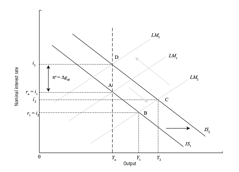
The basic adjustment mechanism is illustrated in Figure 10.1. The economy starts in long-run equilibrium, indicated by point A. Output is at the natural level, and the nominal and the real interest rates are equal, since expected inflation is assumed to be zero. Note that I indicated the long-run equilibrium real interest rate with the symbol r n , since this rate of return is sometimes referred to as the natural real interest rate (i.e. the real interest rate consistent with the long-run equilibrium of the economy). Next, we consider a monetary expansion in the form of an increase in the growth rate of the real money supply, which initially shifts down the LM 1 curve to LM 2 . Assuming that in the very short run inflation expectations are constant, the short-run equilibrium moves to point B,
so that output is above the natural level (Y 1 > Y n ) and both real and nominal interest rates reduced to the lower rates r 1 and i 2 , respectively.

But suppose that the faster money supply growth, once communicated to the public, also causes an increase in inflation expectations above zero. By the Fisher equation, this implies a lower real interest rate for any given nominal rate. The fall in the real interest rate increases demand for investment and shifts the IS curve to the right. The economy moves to the new short-run equilibrium at point C, in which output is even higher (Y 2
> Y 1 ) than after the initial expansion, and the nominal interest rate has returned at least some of the way towards its initial level. In the long run inflation dynamics will restore equilibrium at the natural level of output.

The increase in money growth has no long-run effect on the real interest rate, which returns to r n . This is because money is neutral in the long run so that changes to its growth rate cannot affect the real variable r. But
inflation will rise in the long run, consistent with the faster rate of money growth, and by equation (10.1) this implies a one-for-one increase in the nominal interest rate in the long run. In the diagram this is illustrated by
the economy moving to point D. This long-run result is also known as the Fisher hypothesis, and it is analytically written as:

r n = i – g M

which shows that in the long run the real interest rate equals the difference between the nominal interest rate and the growth rate of the money supply, g M .

The Fisher hypothesis also implies that while the economy adjusts from the short to the long run, the real interest rate must rise in order to return to its natural rate. This is only possible if inflation increases at a rate
higher than the new rate of nominal money growth during the adjustment phase. Under this circumstance, the growth rate of real money is negative and both the nominal and the real interest rates increase at any given
expected inflation rate.

Yield to maturity

A summary measure of the return on a T-year bond is the yield to maturity, defined as the constant interest rate that equates the price of a bond with the present value of the future payments on the bond. The yield on a T-year bond is approximately equal to the average of the current one- year interest rate and the expected one-year rates over the next T–1 years.

Analytically, this is written as:

i T t = (i 1 t + i 1 t + 1 ^e + ... + i 1 T ^e ) / T

which shows that the T-year bond yield is the average between the current and the future expected short-term interest rates.

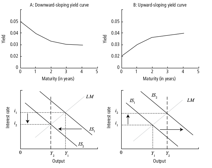
The yield curve, or term structure of interest rates, plots yields against bond maturities. Because the yield is ultimately an average between the current and the future expected short-term interest rates, the yield curve is upward sloping (yields are higher on bonds with longer maturities) when investors expect short-term interest rates to increase in the future. Conversely, the yield curve is downward sloping (yields higher on bonds with shorter maturities) if investors expect short-term interest rates to decline.

Figure 10.2 links the slope of the yield curve to market expectations about future economic activity. Panel A shows that a downward-sloping yield curve may be associated with an expected slowdown in economic activity: when output is above its natural level, the IS curve is expected to shift to the left, leading to a reduction in both output and the interest rate. This implies that the current interest rate is higher than the expected interest rate; hence the yield curve should be downward sloping. Conversely, Panel B shows that an upward-sloping yield curve may be associated, for instance, with an expected recovery in economic activity: when output is below its natural level, the IS curve is expected to shift to the right, leading to an increase in both output and the interest rate. Consequently, financial market participants may expect an increase in the short-term interest rate, hence the positive-sloped yield curve.

The stock market

We begin the description of the stock market by considering the standard three ways in which firms can finance their investment: by issuing bonds (debt finance), by retaining part of their earnings (internal equity finance), and by issuing new shares or stocks (external equity finance). Debt holders or bond holders have contracts (bonds) that promise to pay them a predetermined cash sum at maturity in exchange for cash in the current period. Equity holders or shareholders provide cash to firms in the current period in exchange for control over investment decisions and claims on the residual earnings of the firm in the future.

Firms usually pay dividends to shareholders, which constitute a share of their profits. Broadly speaking, profits are defined as the difference between revenue and cost, and the latter includes also the interest payment on issued bonds. For this reason, the bondholders’ claim on firms’ earnings comes before that of shareholders. In addition, the amount of dividend paid by a firm depends, among other factors, upon its profitability. In this respect, stocks are riskier investments than bonds, since shareholders’ returns are variable and related to firms’ profitability, which varies highly over the business cycle. Many firms do not pay dividends. In this case, shareholders earn a return from their investment only if the resale price of their shares in the future is higher than the current value of their shares.

In the absence of risk, the no-arbitrage condition between bonds and stocks implies that the price of stock is equal to the expected present value of dividends. This result can be illustrated analytically by considering the choice of investing one unit of money in either a bond or a stock for one year. In the first case, the return for the bondholder is equal to 1 + i t . Alternatively, the investor can purchase stock in the current period, receive a dividend in the next year, and then resell the stock. If the current price of the stock is Q t , each unit of money buys 1/ Q t units of stock. The return from holding the stock for one year is given by D t + 1 + Q t + 1 , that is the sum of the expected dividend and the resale price. Therefore, the expected return from investing one unit of money in stock for one year is given by ( D t + 1 + Q t + 1 ) / Q t . The no-arbitrage condition implies that the returns for the bond holder and the shareholder must be the same, so that:

1 + i t = ( D t+1^e + Q t+1 ^e) / Qt

This expression can be solved for Q t as

Q_t = (D_t+1^e/(1 + i_t))(Q_t+1 ^e/(1+1_t)) (10.6)

which shows that the current price of stock is equal to the present value of next year’s dividend and the resale price of the stock. The equilibrium condition in equation (10.6) can be generalised by replacing Q t e + 1 with a
corresponding expression in terms of D t e + 2 and Q t e + 2 , then replacing Q t e + 2 , and so on, that is the present value of the expected stream of dividends plus the present value of the stock T years ahead from t.

The price of a stock in any period t should largely depend upon expectations about the stream of cash flow that the
firm is likely to generate in the future.

In general, news that leads investors to believe that GDP will increase in the future tends to increase stock prices, because higher output means higher profits, and hence higher dividends. News that leads investors to expect a rise in short-term interest rates tends to reduce stock prices, because higher interest rates make investment in bonds more attractive relative to stocks, thereby reducing stock prices.

The current price of stock already reflects all expectations about events occurring in the future. Consequently, future events can only affect stock prices to the extent that they are not fully anticipated by financial market participants. For this reason an anticipated monetary policy should not affect the stock market, whereas unanticipated or unexpected monetary policies can affect it.

The expected present value of future dividends is also referred to as the fundamental value of a stock. This is to highlight that stock prices may sometimes be overpriced or underpriced, to the extent that they deviate from their fundamental value.

A rational speculative bubble occurs when a stock’s price exceeds its fundamental value because investors are willing to pay a high price for it (even with no value) in anticipation of being able to resell it at an even
higher price. This is still consistent with rational behaviour. Even though a crash is possible when stock prices exceed their fundamental value, it makes sense for investors to pay a high price for stocks if they have good reason to believe that prices will increase in the near future.

Deviations of stock prices from their fundamental values which are inconsistent with rational behaviour are, instead, defined as fads.

The Keynesian theory of aggregate investment

Real investment spending includes three broad components:
1. business fixed investment, which refers to plant, machinery, buildings and any equipment purchased by firms for production
2. residential investment, which refers to the purchase of new houses by people to live in and/or to rent
3. inventory investment, which includes all unused or unsold goods stored by firms, such as materials, works in progress and finished products.

The empirical evidence identifies two fundamental facts about investment spending. First, in most industrialised countries business fixed investment represents the largest share of investment spending, followed by residential investment and changes in inventories. Second, investment spending falls substantially during recessions, and by more than consumption does. In this course we will only focus on business fixed investment, and you are not expected to know the determinants of the other two components of investment spending.

Investment spending is a flow variable, whereas physical capital is a stock. In particular, business fixed investment spending refers to the amount spent by firms to add to their stock of capital over a given period. Gross investment measures the total such spending over a given period of time. Net investment measures the net variation of the capital stock after taking into account the loss of capital caused by physical depreciation over the same period of time. Analytically, the relationship between investment and capital defines the fundamental dynamic equation of capital, which is written as:

I t = ∆ K t +1 + δ K

where I t indicates gross investment over period t, ∆ K t + 1 = K t + 1 − K t measures net investment, namely the effective change in physical capital from t to t+1; and the term δK t computes physical depreciation, which
occurs at the constant rate δ.

Keynesian investment theory, assumes aggregate demand for investment to be positively related to the current level of sales, as measured by the current level of GDP, and negatively related to the cost of borrowing, as measured
by the real interest rate. Analytically, the Keynesian investment function is given by:

I t = b 1 Y t – b 2 r t ,

where b 1 and b 2 measure the response of aggregate investment to income and the interest rate.

The Keynesian investment function has the same intrinsic problems as the Keynesian consumption function. First, it is a static function of income, without considering expectations about the future state of the economy. Second, the aggregate value of investment is simply assumed to be related to output and the interest rate, rather than determined by a microfounded model of the economy.

The accelerator model

The accelerator model relates investment spending to fluctuations in aggregate output. There are several versions of the accelerator model, and we will focus on two of them: the simple and the flexible models. The simple accelerator model assumes that there is no depreciation, so that investment spending, I t , is equal to changes in the capital stock, ∆K, which in turn are assumed to be proportional to changes in aggregate output, ∆Y.

Analytically, the simple accelerator model satisfies:
I t = ∆ K t = υ ∆ Y t

where the parameter υ is the accelerator coefficient indicating how much investment firms carry out as a proportion of the variation in output. The accelerator model assumes that firms invest more when demand is increasing over time, ∆ Y t > 0 , whereas they disinvest if output decreases over time ∆ Y t < 0

The most appealing feature of the accelerator model is mainly empirical, since the prescriptions of the model are consistent with the empirical evidence of a strong and positive correlation between changes in output and fluctuations in investment spending. However, the model has several drawbacks. Firms may not have an incentive to invest if they perceive changes in aggregate demand as being temporary rather than permanent. Firms may also increase production following an increase in aggregate demand without increasing investment spending, if they are operating under spare capacity.

In addition, the accelerator model assumes adjustments in the capital stock occur only as a result of changes in current and past demand, while most firms are forward looking and commit to new investment in response to the
expected future levels of demand. However, this latter issue can be handled by assuming that the desired level of capital depends upon the expected future level of demand, Y t+1 ^e. Under this assumption, the model becomes:

K t − K t − 1 = υ ( Y t+1 ^e − Y t ),

The neoclassical model of investment

The neoclassical model provides a dynamic and microfounded theory of aggregate investment. Consider a firm that owns a unit of capital and has to decide how to use it. The firm has two alternatives: either sell the unit of capital at the market price, P kt , or keep it and use it for production. Just as in the analysis of financial investments, we can analyse the firm’s decision between these two alternatives by considering the relative returns associated with them. Selling the capital will yield a total real return of P kt (1 + r t ) in period t + 1. Using it for production will yield extra profits in t + 1, equal to some value that we denote R k1t , plus the value that can be raised by re-selling any capital that still remains, P k e t+1 (l–δ) . Thus it will be relatively profitable to invest if: R k1t + P k e t+1 (l–δ) > P kt (l+r t )

Or: R k1t > r t P kt + δ P k e t+1 – delta P k e t+1

where delta P k e t+1 is the expected change in the price of a unit of capital between t and t + 1. The object on the right-hand side of this expression is sometimes known as the user cost of capital. It is the sum of the interest returns that are sacrificed by a decision to invest in capital, the cost of replacing machinery that will wear out because of its use when investment takes place, and any expected reduction in the price of the capital good between t and t + 1. The inequality states that the returns from investing must at least compensate these three costs.

Clearly, if it is convenient to use one unit of capital in period t, then the firm wonders whether it is also convenient to use a second unit. As for the first unit, the firm compares the expected return from adding a second unit of capital to the existing stock, R k2t , with the expected cost from using that unit.

Under the assumption of the neoclassical production function the return from capital equals the marginal product of capital, which falls as the capital stock rises. Therefore, the return from capital R kt falls as the capital stock increases. This implies that the expected return from the second unit of capital must be lower than the first. More generally, if the cost of capital is constant, the firm must reach a point when adding an extra unit of capital yields an expected return equal to the user cost, so that the firm is indifferent to purchasing that extra unit. In other words there must be a level of the capital stock k * such that:

R k*t = r t P kt + δP kt+1 – ∆P kt+1 (10.10)

Once condition (10.10) is satisfied the firm will not add any extra capital to its existing stock. For this reason, equation (10.10) determines the so-called optimal stock of capital and represents the fundamental investment
criterion followed by firms under the neoclassical model.

Note the striking difference between the Keynesian and the neoclassical investment theories. Under the Keynesian model investment depends upon the current level of output and the current interest rate. Under the neoclassical investment function investment spending depends also on current and expected future levels of output and interest rates, particularly via the impact these have on the expected future price of capital, P kt+1 ^e.

Tobin’s q model of investment

The neoclassical model implies that firms invest in new capital until the optimal capital stock is reached. Because the return from new capital depends upon current and future expected profitability, implicitly the neoclassical model relates investment choices to the value of firms’ capital. Tobin’s q model explicitly relates investment decisions to fluctuations in the stock market. The model argues that the stock market can accurately assess the profitability of investment opportunities that firms face. A firm that has the chance to make higher profits by expanding its capital stock will see this reflected in its share price – even before it has taken any formal decision to invest. In this situation the value of a firm’s shares should exceed the value of the capital that it already has installed – that is, the ‘replacement cost’ of the existing stock. So if the market value of a firm’s capital (its share price) exceeds the replacement cost, the firm can expect to be able to profit from investing.

Analytically, Tobin’s q is thus given by the ratio between the market value and the replacement cost of the capital stock of a firm:

q = Market value of installed capital / Replacement cost of installed capital (10.11)

Note that the q theory assumes that investment choices depend upon the market value of the whole capital in a firm: the existing and the newly installed capital stock. The numerator of q measures the market value of the whole firm. The denominator measures the replacement cost of the same firm, namely how much will it cost to repurchase the whole capital of the firm. For this reason, q in equation (10.11) measures the scale of investment opportunities relative to the firm’s entire capital stock, and is defined as average q.

A link between the neoclassical and the q theories of investment can be established by supposing that a firm holds just one unit of capital, and is considering whether to invest further. The replacement cost of this capital is P kt , its price. The market value of the firm is given by the discounted value of the net returns that this capital will yield:

(1 / (1+r_t)) (R + P e (1–δ))

Tobin’s q is thus given by: q t = (R k1t + P kt+1 (1–δ))/ (P kt (1+r t )) (10.12)

q t >1 is precisely the case in which the returns to capital exceed the user cost, and thus further investment is desirable.

Equation (10.12) defines the so-called marginal q since it relates the market value and replacement cost of just one (marginal) unit of capital. It shows that the optimal capital stock is reached when:

(R k1t + P kt+1 (1–δ)) / (P kt (1+ r t )) = 1

that is the user cost of capital condition in equation (10.10) is satisfied. A q higher than one signals that the actual capital stock is below its optimal value, and firms should increase investment. Vice versa, q < 1 signals that firms have accumulated too much capital, and the best strategy is to reduce the capital stock.

The empirical evidence shows that there is a clear, positive correlation between estimates of Tobin’s q and fluctuations in business investment. This suggests that investment choices, which largely depend upon expected future profits and expected future interest rates, are well understood by stock markets.

More generally, the empirical evidence shows a positive correlation between stock prices and the business cycle. If the replacement cost of capital is fairly stable, a fall in the stock market is, usually, associated with a fall in Tobin’s q, which reflects market pessimism about future capital profitability. In turn, this pessimisim reduces investment spending and, consequently, aggregate demand, output and employment.

Keynesian versus neoclassical theory: the empirical evidence

The Keynesian and neoclassical theories propose two very different views about the determinants of aggregate investment. On the one hand, Keynesian theory argues that investment spending depends upon the current level of aggregate income (profitability) and the interest rate. In sharp contrast, neoclassical theory points out that investors are forward-looking and, thus, they base investment decisions upon their forecasts about future income and interest rates.

Although neoclassical theory provides a more realistic and consistent description of the determinants of investment spending, the empirical evidence suggests two clear patterns that contrast with its predictions.

First, there is strong evidence that the current level of investment is highly correlated with the current level of profits (output). Second, firms with highly profitable investment projects but low current profitability appear to invest too little, as opposed to firms with low profitable investment projects but high current profitability, which appear to invest too much.

There are two main explanations for this conflicting evidence. First, firms with high current profitability are more prone to undertake risky investment projects, since they have the necessary internal funds to cover eventual losses. Second, firms with low current profits must rely more heavily upon debt finance, and are more likely to face borrowing constraints that can prevent them from raising from financial markets the necessary funds to invest.

Blanchard, O., Johnson, D.R., (2013) Macroeconomics (sixth edition), Pearson

Chapter 14: Expectations The Basic Tools

14-1 Nominal versus Real Interest Rates

Interest rates expressed in terms of dollars (or, more generally, in units of the national currency) are called nominal interest rates. The interest rates printed in the financial pages of newspapers are nominal interest rates.

Interest rates expressed in terms of a basket of goods are called real interest rates.

One plus the real interest rate equals the ratio of one plus the nominal interest rate, divided by one plus the expected rate of inflation.

(1 + r_t ) = (1 + i_t) / (1 + p^e_t+1)

The real interest rate is (approximately) equal to the nominal interest rate minus expected inflation.
r_t ~= i_t - p^e_t+1

* When expected inflation equals zero, the nominal and the real interest rates are equal.
* Because expected inflation is typically positive, the real interest rate is typically lower than the nominal interest rate.
* For a given nominal interest rate, the higher the expected rate of inflation, the lower the real interest rate.

Deflation was a major issue in the Great Depression.

14-2 Nominal and Real Interest Rates, and the IS–LM Model

In the IS–LM model we developed in the core (Chapter 5), “the” interest rate came into play in two places: It affected investment in the IS relation, and it affected the choice between money and bonds in the LM relation

Take the IS relation first. Our discussion in Section 14-1 makes it clear that firms, in deciding how much investment to undertake, care about the real interest rate. So what belongs in the IS relation is the real interest rate. Let r denote the real interest rate. The IS relation must therefore be modified to read:

Y = C (Y - T) + I (Y, r) + G

Investment spending, and thus the demand for goods, depends on the real interest rate.

Now turn to the LM relation. When we derived the LM relation, we assumed that the demand for money depended on the interest rate. This is the nominal interest rate. Remember why the interest rate affects the demand for money. When people decide whether to hold money or bonds, they take into account the opportunity cost of holding money rather than bonds - opportunity cost is what they give up by holding money rather than bonds. Money pays a zero nominal interest rate. Bonds pay a nominal interest rate of i. Hence, the opportunity cost of holding money is equal to the difference between the interest rate from holding bonds minus the interest from holding money, so i - 0 = i, which is just the nominal interest rate. Therefore, the LM relation is still given by:

M/P = YL(i)

* The interest rate directly affected by monetary policy (the interest rate that enters the LM equation) is the nominal interest rate.
* The interest rate that affects spending and output (the rate that enters the IS rela-tion) is the real interest rate

14-3 Money Growth, Inflation, Nominal and Real Interest Rates

Does higher money growth lead to lower interest rates, or does higher money growth lead to higher interest rates? The answer: Both!

There are two keys to the answer: one, the distinction we just introduced between the real and the nominal interest rate; the other, the distinction between the short run and the medium run. As you shall see, the full answer is:

* Higher money growth leads to lower nominal interest rates in the short run but to higher nominal interest rates in the medium run.
* Higher money growth leads to lower real interest rates in the short run but has no effect on real interest rates in the medium run.

The IS curve is still downward sloping: For a given expected rate of inflation (p^e), the nominal interest rate and the real interest rate move together. So, a decrease in the nominal interest rate leads to an equal decrease in the real interest rate, leading to an increase in spending and in output.

The LM curve is upward sloping: Given the money stock, an increase in output, which leads to an increase in the demand for money, requires an increase in the nominal interest rate.

The equilibrium is at the intersection of the IS curve and the LM curve, point A, with output level Y A , nominal interest rate i A . Given the nominal interest rate, the real interest rate r A is given by r A = i A - p e .

Assume the economy is initially at the natural rate of output, so Y A = Y n. Now suppose the central bank increases the rate of growth of money. What happens to output, to the nominal interest rate, and to the real interest rate in the short run?

An increase in money growth increases the real money stock in the short run. This increase in real money leads
to an increase in output and decreases in both the nominal and real interest rates.

Turn now to the medium run. Suppose that the central bank increases the rate of money growth permanently. What will happen to output and nominal and real interest rates in the medium run?

In the medium run, output returns to the natural level of output, Yn. In the medium run, the real interest rate returns to the natural interest rate, r n . It is independent of the rate of money growth. In the medium run, the rate of inflation is equal to the rate of money growth.

In the medium run, the nominal interest rate is equal to the natural real interest rate plus the rate of money growth. So, in the medium run, an increase in money growth leads to an equal increase in the nominal interest rate.

This result—that, in the medium run, the nominal interest rate increases one-for-one with inflation—is known as the Fisher effect, or the Fisher hypothesis.

Because low interest rates lead to higher demand, which leads to higher output, which eventually leads to higher inflation; higher inflation leads in turn to a decrease in the real money stock and an increase in interest rates.

An increase in money growth leads initially to decreases in both the real and the nominal interest rates. Over time, however, the real interest rate returns to its initial value and the nominal interest rate rises to a new higher value, equal to the initial value plus the increase in money growth.

14-4 Expected Present Discounted Values

The expected present discounted value of a sequence of future payments is the value today of this expected sequence of payments.

If the one-year nominal interest rate is i t , lending one dollar this year implies getting back 1 + i t dollars next year. Equivalently, borrowing one dollar this year implies paying back 1 + i t dollars next year. In this sense, one dollar this year is worth 1 + i t dollars next year.

More formally, we say that 1> 1 1 + i t 2 is the present discounted value of one dollar next year. The word “present” comes from the fact that we are looking at the value of a payment next year in terms of dollars today. The word “discounted” comes from the fact that the value next year is discounted, with 1> 11 + i t 2 being the discount factor (The one-year nominal interest rate, i t , is sometimes called the discount rate).

“Expected present discounted value” is a heavy expression to carry; instead, for short, we will often just use present discounted value, or even just present value.

We can compute the present value of a sequence of payments in two ways. One way is to compute it as the present value of the sequence of payments ex- pressed in dollars, discounted using nominal interest rates, and then divided by the price level today. The other way is to compute it as the present value of the sequence of payments expressed in real terms, discounted using real interest rates. The two ways give the same answer.

Summary
* The nominal interest rate tells you how many dollars you need to repay in the future in exchange for one dollar today.
* The real interest rate tells you how many goods you need to repay in the future in exchange for one good today.
* The real interest rate is approximately equal to the nominal interest rate minus expected inflation.
* Investment decisions depend on the real interest rate. The choice between money and bonds depends on the nominal interest rate. Thus, the real interest rate enters the IS relation, while the nominal interest rate enters the LM relation.
* In the short run, an increase in money growth decreases both the nominal interest rate and the real interest rate. In the medium run, an increase in money growth has no effect on the real interest rate, but it increases the nominal interest rate one-for-one.
* The proposition that, in the medium run, changes in inflation are reflected one-for-one in changes in the nominal interest rate is known as the Fisher effect or the Fisher hypothesis. The empirical evidence suggests that, while it takes a long time, changes in inflation are eventually re-
flected in changes in the nominal interest rate.
* The expected present discounted value of a sequence of payments equals the value this year of the expected sequence of payments. It depends positively on current and future expected payments and negatively on current and future expected interest rates.
* When discounting a sequence of current and expected future nominal payments, one should use current and expected future nominal interest rates. In discounting a sequence of current and expected future real payments, one should use current and expected future real interest rates.

Chapter 15: Financial Markets and Expectations

15-1 Bond Prices and Bond Yields

Bonds differ in two basic dimensions:

Default risk: The risk that the issuer of the bond (it could be a government or a company) will not pay back the full amount promised by the bond.

Maturity: The length of time over which the bond promises to make payments to the holder of the bond. A bond that promises to make one payment of $1,000 in six months has a maturity of six months; a bond that promises to pay $100 per year for the next 20 years and a final payment of $1,000 at the end of those 20 years has a maturity of 20 years.

Bonds of different maturities each have a price and an associated interest rate called the yield to maturity, or simply the yield. Yields on bonds with a short maturity, typically a year or less, are called short-term interest rates. Yields on bonds with a longer maturity are called long-term interest rates.

The yield to maturity on an n-year bond, or, equivalently, the n-year interest rate, is defined as that constant annual interest rate that makes the bond price today equal to the present value of future payments on the bond.

15-2 The Stock Market and Movements in Stock Prices

But while governments finance themselves by issuing bonds, the same is not true of firms. Firms finance themselves in three ways. First, and this is the main channel for small firms, through bank loans debt finance—bonds and loans; and third, through equity finance, issuing stocks—or shares, as stocks are also called. Instead of paying predetermined amounts as bonds do, stocks pay dividends in an amount decided by the firm. Dividends are paid from the firm’s profits. Typically dividends are less than profits, as firms retain some of their profits to finance their investment. But dividends move with profits.

Two equivalent ways of writing the stock price: The—nominal—stock price equals the expected present discounted value of future nominal dividends, discounted by current and future nominal interest rates.

The—real—stock price equals the expected present discounted value of future real dividends, discounted by current and future real interest rates.

Summary

* Arbitrage between bonds of different maturities implies that the price of a bond is the present value of the payments on the bond, discounted using current and expected short-term interest rates over the life of the bond. Hence, higher current or expected short-term interest rates lead to lower
bond prices.
* The yield to maturity on a bond is (approximately) equal to the average of current and expected short-term interest rates over the life of a bond.
* The slope of the yield curve—equivalently, the term structure—tells us what financial markets expect to happen to short-term interest rates in the future. A downward-sloping yield curve (when long-term interest rates are lower than short-term interest rates) implies that the market expects
a decrease in short-term interest rates; an upward-sloping yield curve (when long-term interest rates are higher than short-term interest rates) implies that the market expects an increase in short-term rates.
* The fundamental value of a stock is the present value of expected future real dividends, discounted using current and future expected one-year real interest rates. In the absence of bubbles or fads, the price of a stock is equal to its fundamental value.
* An increase in expected dividends leads to an increase in the fundamental value of stocks; an increase in current and expected one-year interest rates leads to a decrease in their fundamental value.
* Changes in output may or may not be associated with changes in stock prices in the same direction. Whether they are or not depends on (1) what the market expected in the first place, (2) the source of the shocks, and (3) how the market expects the central bank to react to the output change.
* Asset prices can be subject to bubbles and fads that cause the price to differ from its fundamental value. Bubbles are episodes in which financial investors buy an asset for a price higher than its fundamental value, anticipating to resell it at an even higher price. Fads are episodes in
which, because of excessive optimism, financial investors are willing to pay more for an asset than its fundamental value.