2.1 Introduction

By the end of this chapter, the Essential reading and activities, you should be able to:
* explain the implications of the assumptions on the consumer’s preferences
* describe the concept of modelling preferences using a utility function
* draw indifference curve diagrams starting from the utility function of a consumer
* draw budget lines for different prices and income levels
* solve the consumer’s utility maximisation problem and derive the demand for a
* consumer with a given utility function and budget constraint
* analyse the effect of price and income changes on demand
* explain the notion of a compensated demand function
* explain measures of the welfare impact of a price change: change in consumer
* surplus, equivalent variation and compensating variation, and use these measures
* to analyse the welfare impact of a price change in specific cases
* construct the market demand curve from individual demand curves
* explain the notion of elasticity of demand
* analyse the decision to supply labour
* analyse the problem of savers and borrowers
* derive the present discounted value of payment streams and explain bond pricing.

2.2 Overview of the chapter

We start by analysing preferences, utility and choice. Next, we learn how to construct demand curves, and analyse their properties. We also explain various welfare measures. We then analyse the labour supply decision of an individual before moving on to saving and borrowing with two periods. Finally, we learn to carry out present value calculations with many periods and analyse bond pricing.

2.3 Preferences, utility and choice

Preferences and Utility

The theory of choice starts with rational preferences. Generally, preferences are primitives in economics – you take these as given and proceed from there. To be able to create a model of choice that has some predictive power, we do need to put some restrictions on preferences to rule out irrational behaviour. A utility function is an artificial concept – no-one actually has a utility function.

Preferences generally give us rankings among bundles rather than some absolute measure of satisfaction derived from bundles. Preferences typically give us an ‘ordinal’ ranking among bundles of goods. Since utility is simply a representation of preferences, it is also an ordinal measure.

Indifference Curves

Once we can represent preferences using a continuous utility function, we can draw indifference curves. An indifference curve is the locus of different bundles of goods that yield the same level of utility. In other words, an indifference curve for utility function u(x, y) is given by u(x, y) = k, where k is some constant. As we vary k, we can trace out the indifference map.

Previously, we put some restrictions on preferences. What do these restrictions imply for indifference curves? We have the following properties:

1. If an indifference curve is further from the origin compared to another indifference curve, any point on the former is preferred to any point on the latter (implied by the assumption that more is better).
2. Indifference curves cannot slope upwards (implied by more is better).
3. Indifference curves cannot be thick (again, implied by more is better).
4. Indifference curves cannot cross (implied by transitivity).
5. Every bundle of goods lies on some indifference curve (follows from completeness).

A further important property concerns the rate at which a consumer is willing to substitute one good for another along an indifference curve. The marginal rate of substitution of a consumer between goods x and y is the units of y the consumer is willing to substitute (i.e. willing to give up) to obtain one more unit of x.

dy / dx uconstant = − (MU x / MU y)

The marginal rate of substitution is the absolute value of the slope:

MRS xy = MU x/ MU y

Budget Constraint

Once we have specified our model of preferences, we need to know the set of goods that a consumer can afford to buy. This is captured by the budget constraint. Since consumers are generally taken to be price-takers (i.e. what an individual consumer purchases does not affect the market price for any good), the budget line is a straight line.

Utility Maximisation

The consumer chooses the most preferred point in the budget set. If preferences are such that indifference curves have the usual convex shape, the best point is where an indifference curve is tangent to the budget line. If indifference curves satisfy the usual convexity property, there is an interior tangency point with the budget constraint line at which the maximum utility is attained.

Note that the ‘more is better’ assumption ensures that a consumer spends all income (if not, then the consumer could increase utility by buying more of either good). Therefore, the budget constraint is satisfied with equality. It follows that the consumer maximises u(x, y) subject to the budget constraint P_x x + P_y y = M.

The first-order conditions above are, by themselves, not sufficient to guarantee a maximum. We also need the second-order condition to hold. It is better to derive this formally once you have learned matrix algebra, which allows a relatively simple exposition of the second-order condition. For our purposes here, note that the diminishing MRS condition is sufficient to guarantee that a maximum occurs at the point satisfying the first-order conditions. This should also be clear to you from the graph. If indifference curves satisfy the usual convexity property, there is an interior tangency point with the budget constraint line at which the maximum utility is attained.

The maximisation exercise above gives us the demand for goods x and y at given prices and income.

Elasticities of demand

The classification of goods according to the response of demand to income changes.

Normal goods: a consumer buys more of these when income increases.
Inferior goods: a consumer buys less of these when income increases.

Note that it is not possible for all goods to be inferior. This would violate the ‘more is
better’ assumption.

The income-consumption curve of a consumer traces out the path of optimal bundles as income varies (keeping all prices constant). Using this exercise, we also plot the relationship between quantity demanded and income directly. The curve that shows this relationship is called the Engel curve.

Elasticities of demand

The notion of elasticity of demand captures the responsiveness of demand to variables such as prices and income.

This is the percentage change in quantity demanded of a good in response to a given percentage change in the price of the good, given by:

ε = dQ/Q/dP/P = P dQ /Q dP

Note that ε < 0 since demand is typically downward-sloping. Demand is said to be elastic if ε < −1, unit elastic if ε = −1, and inelastic if ε > −1.

Income elasticity. Denoting income by M , income elasticity of demand is given by:
ε M/M = P dM/dP.

This is positive for normal goods, and negative for inferior goods. When ε M exceeds 1, we call the good a luxury good. Necessities like food have income elasticities much lower than 1.

Cross-price elasticity: demand for good i with respect to the price of good j.

ε ij = (P j/Q i)(dQ i/dP j)

This is negative for complements and positive for substitutes.

The compensated demand curve

To derive the demand function for good x, we vary the price of good x but hold constant the prices of other goods and income. As the price changes so that the optimal choice changes, the utility of the consumer at the optimal point also changes. This is the usual demand curve, and is also known as the Marshallian demand curve, or the uncompensated demand curve.

A compensated, or Hicksian, demand curve can be derived as follows. Suppose as the price of a good changes, we keep utility constant while allowing income to vary. In other words, if the price of x, say, falls (so that the new optimal bundle of the consumer would be associated with a higher level of utility if income is left unchanged), we take away enough income to leave the consumer at the original level of utility. It is clear that this process eliminates the income effect and simply captures the substitution effect.

Some properties of compensated demand curves.

* A compensated demand curve always slopes downwards.
* For a normal good, the compensated demand curve is less elastic compared to the uncompensated demand curve.
* For an inferior good, the compensated demand curve is more elastic compared to the uncompensated demand curve

Welfare measures: ∆CS, CV and EV

When drawing demand curves, we typically draw the inverse demand curve (price on the vertical axis, quantity on the horizontal axis). In such a diagram, the consumer surplus (CS) is the area under the (inverse) demand curve and above the market price up to the quantity purchased at the market price. This is the most widely-used measure of welfare. We can measure the welfare effect of a price rise by calculating the change in CS (denoted by ∆CS).

However, ∆CS is not an exact measure because of the presence of an income effect. Ideally, we would use the compensated demand curve to calculate the welfare change. CV is the amount of money that must be given to a consumer to offset the harm from a price increase, i.e. to keep the consumer on the original indifference curve before the price increase. EV is the amount of money that must be taken away from a consumer to cause as much harm as the price increase. In this case, we keep the price at its original level (before the rise) but take away income to keep the consumer on the indifference curve reached after the price rise.

Compensating variation (CV)
CV is the amount of money that must be given to a consumer to offset the harm from a price increase, i.e. to keep the consumer on the original indifference curve before the price increase

Equivalent variation (EV)
EV is the amount of money that must be taken away from a consumer to cause as much harm as the price increase. In this case, we keep the price at its original level (before the rise) but take away income to keep the consumer on the indifference curve reached after the price rise.

For a normal good, we have CV > ∆CS > EV, and for an inferior good we have CV < ∆CS < EV. The measures would coincide for preferences that exhibit no income effect.

2.5 Labour supply

Every economic agent has, in a day, 24 hours. An agent must choose how many of these hours to spend working, and how many hours of leisure to enjoy. Working earns the agent income, which represents all goods the agent can consume. But the agent also enjoys leisure. If the hourly wage is w, this can be seen as the price that the agent must pay to enjoy an hour of leisure.

The agent, therefore, faces the following problem. Let Z denote the number of hours worked, N denote the number of leisure hours, M denote income and M̄ denote unearned income (inheritance, gifts etc).

max u(N, M ); subject to: Z = 24 − N, M = wZ + M̄ .

We can simplify the constraints to M = w(24 − N ) + M̄ , or M + wN = 24w + M̄ .

Income Effect
If the hourly wage is w, this can be seen as the price that the agent must pay to enjoy an hour of leisure. The rise in w raises income at current levels of labour and leisure. Assuming leisure is a normal good (this should be your default assumption), this raises the demand for leisure.

Substitution effect
The rise in w makes leisure relatively more expensive, causing the agent to substitute away from leisure. This reduces demand for leisure.

The two effects go in opposite directions, therefore the direction of the total effect is unclear. In most cases, the substitution effect dominates, giving us an upward-sloping labour supply function. However, it is possible, especially at high levels of income (i.e. when wage levels are high), that the income effect might dominate. In that case we would get a backward-bending labour supply curve which initially slopes upward but then turns back and has a negative slope

If leisure is, on the other hand, an inferior good, the two effects would go in the same
direction and labour supply would necessarily slope upwards.

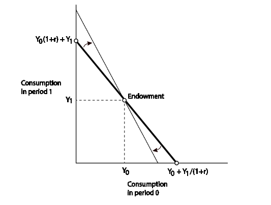
2.6 Saving and borrowing: intertemporal choice

We focus on a two-period problem. Suppose the agent’s endowment is Y 0 in period 0 and Y 1 in period 1. Given a rate of interest r, the present value of income in period 0 is Y 0 + Y 1 /(1 + r). If the individual consumes all income in period 0, C 0 is equal to this present value, and C 1 = 0. If all income is saved for period 1, then income at period 1 is (1 + r)Y 0 + Y 1 . In this case, C 1 is this amount and C 0 = 0. Therefore, we have C 1 = (Y 0 − C 0 )(1 + r) + Y 1 , which gives us the intertemporal budget constraint. The problem is then as follows:

max u(C 0 , C 1)

subject to the intertemporal budget constraint: C0 + ( C1 / (1+r)) = Y0 + (( Y1 / (1 +r))

This is similar to a standard optimisation problem with two goods, C 0 and C 1 , where
the price of the former is 1 and the price of the latter is 1/(1 + r).

Unsurprisingly, the optimum satisfies the property that:

(MU_C0/ MU_C1) = 1 +r

If the optimal consumption bundle is C 0 = Y 0 and C 1 = Y 1 , the agent is neither a saver
nor a borrower. If C 0 > Y 0 the agent is a borrower, and if C 0 < Y 0 the agent is a saver
(lender). How does a change in r alter behaviour?

From the borrower's perspective.

Income effect
For a borrower, Y0 < C0, so that a rise in the interest rate lowers income tomorrow. Given consumption is normal in both periods, the agent should consume less in period 0 (borrow less).

Substitution effect
A rise in the interest rate makes immediate consumption more costly. Therefore, the substitution effect suggests that the individual should choose to lower C0 and, therefore, borrow less.

Since the two effects go in the same direction, the direction of change is unambiguous: a
rise in the rate of interest lowers borrowing.

From the lender's perspective:

Income effect
For a saver, Y 0 > C 0 , so that a rise in the interest rate raises income tomorrow. Given
consumption is normal in both periods, the agent should consume more in period 0 (save less).

Substitution effect
A rise in the interest rate makes immediate consumption more costly. Therefore, the substitution effect suggests that the individual should choose to lower C 0 (save more).

Since the two effects go in opposite directions, the total effect on saving is uncertain.
Usually, the substitution effect dominates so that agents save less when the interest rate
rises, but it could go the other way.

2.7 Present value calculation with many periods

The previous section discussed the calculation of present value for a two-period stream of payoffs. We can extend this easily to multiple (or infinite) periods.

Suppose we have a stream of payoffs y 0 , y 1 , . . . , y n in periods 0, 1, . . . , n, respectively.
Suppose the rate of interest is given by r. The present value in period 0 of this stream
of payoffs is given by:

PV = y_0 + ((y_1 /(1 + r)) + ((y_1 /(1 + r)^2) + ... + ((y_n /(1 + r)^n)

If we write δ = 1/(1 + r), we can write this as: PV = y 0 + δy 1 + δ 2 y 2 + · · · + δ n y n .

Bonds

A bond typically pays a fixed coupon amount x each period (next period onwards) until a maturity date T , at which point the face value F is paid. The price of the bond, P , is simply the present value given by the above PV.

P = δx + δ 2 x + · · · + δ T F.

Note that the price declines if δ falls, which happens if r rises. The price of a bond has an inverse relationship with the rate of interest.

A special type of bond is a consol or a perpetuity that never matures.

Reading: Nicholson, W., Intermediate Microeconomics and its application (sixth edition), Dryden Press, 1994

Chapter Three: The Economic Theory of Choice

Theory of Choice [is] the interaction of preferences and income that cause people to make the choices that they do... modeled using the concept of utility... the satisfaction that a person receives from his or her activities. p59

Ceteris paribus assumption. In economic analysis, holding all other factors constant so that only the factor being studied is allowed to change p59

The utility in a two-good economy can be compared in functional notation

Utility = U(X, Y; other things)

Complete preferences [are] the assumption that an individual is able to state which of any two preferences are preferred. p62
Transitivity of preferences [is] The property that is A is preferred to B, and B is preferred to C, then A must be preferred to C. p63

Indifference curve [is] All the combinations of goods and services that provide the same level of utility. p64

Marginal rate of substitution (MRS) [is] the rate at which an individual is willing to reduce consumption of one good when he or she gets one more until of another good remaining equally well-off. The negative of the slope of an indifference curve. p65

Indifference curve map [is] a contour map that shows the utility an individual obtains form all possible consumption options. p68

Illustrations of specific preferences p70

Useless Good. Smoke grinders (Y), Food per week (X), Vertical line
Economic Bad. Houseflies (Y), Food per week (X), upwards sloping
Perfect Substitute. Exxon Oil (Y), Mobil Oil (X), downwards strait slope 1:1
Perfect complement. Right shoes (Y), Left shoes (X), vertical line right angle, horizontal line.

Budget constraint. The limit that income places on the combination of goods and services that an individual can buy. p74 Separates affordable and unaffordable regions.

Slope of budget constraint = slope of indifference curve

Px/Py = MRS (neglecting that both slopes are negative)

Common representation is square root measurement of utility. Utility = U(X,Y) = sqrt(X*Y) p80

(Maximum utility tends to the middle of the distribution due to diminishing returns of goods)

Composite good [is] Combining expenditures on several different goods whose relative prices do not change into a single good for convenience in analysis. p85

Chapter 4

Homongeneous demand function: Quantity demanded does not change when prices and income increase in the same proportion (no really?!)

Normal good: A good that is bought in greater quantities as income increases.
Inferior good: A good that is bought in lesser quantities as income increases.

Substitution effect. The part of the change in quantity demanded that is caused by substitution of one good for another. A movement along an indifference curver.

Income effect. The part of change in quantity demanded that is caused by a change in real income.

Income effect and substitution effect are combined for changes in indifference.

Giffen's paradox: (Might not actually exist, anaedoctal story) Price increases and people buy *more* of a good.

Lump-sum principle: A broad based tax has less cost that a targetted one. A targetted tax reduces purchasing power *and* redirects purchasing. Sometimes (e.g., carbon tax) you might want this.

Complements: Two goods such that if the prices of one increases the demand for the other decreases.

Substitutes: Two goods such that if the price of one increases the demand for the other increases.

Individual demand curve; a graphic representation of the relationship between the price of a good and the quantity of it demanded for each good and each individual. Note shape of demand curve depending on elasticity; water is very inelastic, food - as a generic good - is inelastic. Note however if it is a major portion of income demand may still decline as people will do without.

An increase or decrease in the quantity demanded is a movement along a demand curve.

An increase or decrease in demand is a shift in the entire demand curve.