3.1 Introduction

In the previous chapter, we studied consumer choice in environments that had no element of uncertainty. However, many important economic decisions are made in situations involving some degree of risk. In this chapter, we cover a model of decision-making under uncertainty called the expected utility model. The model introduces the von Neumann–Morgenstern (vN–M) utility function. This is unlike the ordinal utility functions we saw in the previous chapter and has special properties. In particular, the curvature of the vN–M utility function can indicate a consumer’s attitude towards risk. Once we introduce the model, we use it to derive the demand for insurance and also introduce a measure of the degree of risk aversion.

By the end of this chapter, the Essential reading and activities, you should be able to:

* calculate the expected value of a gamble
* explain the nature of the vN–M utility function and calculate the expected utility from a gamble
* explain the different risk attitudes and what they imply for the vN–M utility function
* analyse the demand for insurance and show the relationship between insurance and premium
* explain the concept of diversification
* calculate the Arrow–Pratt measure of risk aversion for different specifications of the vN–M utility function.

Random variable
A variable that represents the outcomes from a random event. A random variable has many possible values, and each value occurs with a specified probability.

Expected value of a random variable

Suppose X is a random variable that has values x 1 , . . . , x n . For each i = 1, 2, . . . , n,
the value x i occurs with probability p i , where p 1 + p 2 + · · · + p n = 1. The expected
(or ‘average’) value of X is given by:

E(X) = p 1 x 1 + p 2 x 2 + · · · + p n x n = Sum p i x i

3.4 Expected utility theory

Expected utility theory was developed by John von Neumann and Oscar Morgenstern in their book The Theory of Games and Economic Behavior. (Princeton University Press, 1944; expected utility appeared in an appendix in the second edition in 1947).

Suppose an agent faces a gamble G that yields an amount x_1 with probability p_1 , x_2 with probability p_2 , . . . , and x_n with probability p_n . How should the agent evaluate this gamble? They showed that under their axioms, there exists a function u such that the gamble can be evaluated using the following ‘expected utility’ formulation:
E(U (G)) = p_1 u(x_1 ) + p_2 u(x_2 ) + · · · + p n_u(x_n ).

The function u is known as the von Neumann–Morgenstern (vN–M) utility function. The vN–M utility function is somewhat special. It is not entirely an ordinal function like the utility functions you saw in the last chapter. Starting from a vN–M u function, we can make transformations of the kind a + bu, with b > 0 (these are called positive affine transformations), without changing the expected utility property but not any other kinds of transformations (for example, u 2 is not allowed). The reason is that, as we discuss below, the curvature of the vN–M utility function captures attitude towards risk. Transformations other than positive affine ones change the curvature of this function, and therefore the transformed u function would not represent the same risk-preferences as the original. Thus vN–M utility functions are partly cardinal.

3.5 Risk aversion

We can show that an agent with a concave vN–M utility function over wealth is risk-averse. Let us show this by establishing that an agent with a concave u function would reject a fair gamble.

Recall that a function f (W ) is concave if f 00 (W ) < 0, i.e. the second derivative of the
function with respect to W is negative.

Suppose G is a gamble which yields 20 with probability 1/2, and 10 with probability 1/2. Suppose an agent has wealth 15 and is given the following choice: invest 15 in gamble G, or do nothing. Note that the expected value of the gamble, E(G), is exactly 15, so that this is a fair gamble (the expected wealth is the same whether G is accepted or rejected).

3.6 Risk aversion and demand for insurance

A risk-averse individual would pay to obtain insurance. To see that, it is useful to define the certainty equivalent (CE) of a gamble. The CE of a gamble is the certain wealth that would make an agent indifferent between accepting the gamble and accepting the certain wealth. The CE is lower than the expected income of 10. Suppose an agent simply faced gamble G (i.e. did not have the choice between G and 10, but simply faced G). Clearly, since the CE is lower than the expected outcome of G, this agent would be willing to pay a positive amount to buy insurance. How much would the agent be willing to pay? The amount an agent pays for insurance is called the risk premium.

A vN–M utility function is given by: u(W) = √W

e.g., with probability 0.5 wealth is 100, and with probability 0.5 a loss occurs so that wealth becomes 64.

This is given by:

E(U ) = 0.5 × √100 + 0.5 × √64 = 9.

W is a concave function

The maximum premium to pay to buy full insurance: Calculate the certainty equivalent of the gamble

u(CE) = E(U ), √CE = 9, implying that CE = 81. Therefore, the maximum premium is 100 − 81 = 19.

The minimum premium. Assuming the insurance company is risk-neutral, it must break even. So the minimum premium (or fair premium) is R min such that it equals the expected payout, which is 0.5 × (100 − 64) = 18. (Note that this is simply 100 − E(W ), where E(W ) is expected wealth, which is 82 in this case.)

If insurance is fair, it does not matter what the degree of risk-aversion is. Every risk-averse agent would buy full insurance. If, on the other hand, the insurance premium is greater than the fair level, how much insurance an agent buys depends on their degree of risk-aversion. No agent with a finite degree of risk-aversion would buy full insurance anymore, but the extent of insurance purchased increases as the agent’s degree of risk-aversion rises.

Suppose a risk-averse agent has wealth W , but faces the prospect of a loss of L with probability p, where 0 < p < 1. The agent can buy a coverage of X by paying the premium rX.

The wealth if loss occurs is given by W L = W − L + X − rX, and the wealth when no loss occurs is given by W N = W − rX. The expected utility of the agent is:

E(U ) = pu(W − L + X − rX) + (1 − p)u(W − rX) = pu(W L ) + (1 − p)u(W N ).

Maximising with respect to X, we get the first-order condition:
pu' (W L )(1 − r) − (1 − p)u' (W N )r = 0.

3.7 Risk-neutral and risk-loving preferences

Just as a concave vN–M utility function represents risk aversion, the opposite – a convex vN–M utility function (so that we have u'' > 0) – represents risk-loving behaviour, and the vN–M utility function is a straight line (u'' = 0) for a risk-neutral agent.

A risk-neutral agent does not care about risk and only cares about the expected value of a gamble. In other words, a risk-neutral agent is indifferent between accepting and rejecting a fair gamble. For a risk-neutral agent, we can write the vN–M utility function of wealth simply as:
u(W ) = W.

3.8 The Arrow–Pratt measure of risk aversion

We discussed different degrees of risk aversion in the section above. How do we measure the degree of risk aversion? As you might guess, the degree of risk aversion has to do with the curvature of the vN–M utility function u. The more concave it is, the greater the degree of risk aversion. The closer it is to a straight line, the lower the degree of risk aversion. Since the second derivative captures the curvature, a measure of risk aversion might be u''.

However, this would not be ideal for the following reason. We know that a positive affine transformation of u, say u b = a + bu, where a and b are positive constants, does not change attitude towards risk. But such a transformation would change the second derivative and, therefore, change the risk measure. This problem could be avoided if u'' is divided by u' . Furthermore, since the most common risk attitude is risk aversion, and for this case u'' < 0, putting a negative sign in front of u'' would deliver a positive risk measure under risk aversion. These help to interpret the Arrow–Pratt measure of risk aversion, which is given by:

ρ = − (u''/u')

That is, the Arrow–Pratt measure of risk aversion is −1 times the ratio of the second derivative and the first derivative of the vN–M utility function. This is the most common measure of risk aversion.

3.9 Reducing risk

Insurance provides a way to reduce risk. Diversification is also another way to reduce risk.

Reading: Nicholson, W., Synder, C., Intermediate Microeconomics and its application (eleventh edition), South-Western, Cengage Learning, 2010

Chapter 4: Uncertainty

Two statistical concepts that originated from studying gambles of chance, probability and expected value, are very important to our study of economic choices in uncertain situations.
p139

Probability: The relative frequency with which an event occurs.
Expected value : The average outcome from an uncertain gamble.
Fair gamble: Gamble with an expected value of zero. p140

Risk aversion: The tendency of people to refuse to accept fair gambles. p142

Bernoulli [identified risk aversion] (and most later economists) assumed that the utility associated with the payoffs in a risky situation increases less rapidly than the dollar value of these payoffs. That is, the extra (or marginal) utility that winning an extra dollar in prize money provides is assumed to decline as more dollars are won. p142

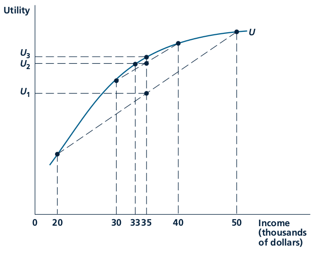
Diminishing marginal utility of payoff

Choosing among Gambles
To solve problems involving a consumer’s choice over gambles, you should proceed in two steps. First,
using the formula for expected values, compute the consumer’s expected utility from each gamble.
Then choose the gamble with the highest value of this number. p143

The less U bends (that is, the more linear U is), the less risk averse is the person. In the extreme, if U is a straight line, then the person will be indifferent between a certain outcome and a gamble with the same expected payoff. In other words, he or she would accept any fair gamble. A person with these risk preferences is said to be risk neutral. p144

Fair insurance: Insurance for which the premium is equal to the expected value of the loss. p146

Risk-averse individuals will always buy insurance against risky outcomes unless insurance premiums exceed the expected value of a loss by too much. p146

Those who expect large losses will buy insurance, whereas those who expect small ones will not. This adverse selection results in the insurer paying out more in losses than expected unless the insurer finds a way to control who buys the policies offered. p146

Diversification
A second way for risk-averse individuals to reduce risk is by diversifying p147

Diversification: The spreading of risk among several alternatives rather than choosing only one. p149