5.1 Introduction

Over the next few chapters we develop models to analyse different market structures. In particular, we analyse two extremes: a competitive market and a monopoly. Later on we also analyse oligopoly. To develop these models, we need to make use of a variety of concepts on the nature of technology, costs and optimisation by firms. This chapter introduces various concepts to this end, many of which you should already be familiar with from previous courses.

This chapter aims to introduce a variety of concepts and calculations that can be used to analyse the production decisions of firms under a variety of market structures.

* explain the concepts of average and marginal product and their relationship
* derive the optimal input purchasing decision of a firm in the short run
* derive the optimal input mix decision in the long run
* explain the concepts of isoquants and marginal rate of technical substitution
* explain how the shape of isoquants depends on input substitutability
* explain the concepts of marginal cost, average cost, fixed cost, sunk cost and variable cost
* explain the various cost curves faced by a firm in the short run and in the long run
* derive the profit-maximising output of a firm
* explain the shut-down decision of a firm.

5.3 A general note on costs

The term ‘cost’ in economics – wherever it occurs – refers to opportunity cost. In other words, the cost of a resource is measured by how much value it would add in its next best use. This is often different from how an accountant would view the costs of a firm. In coming up with a figure for the annual costs of an owner-managed firm an accountant would typically add up the expenses on various categories, but would not include the opportunity cost of the work that the owner has put in or the opportunity cost of own funds that the owner might have invested in the firm. However, for an economist, these are costs just as wages to employees are costs. In sum, the notion of opportunity cost tries to capture the true underlying cost of all factors, rather than costs that are useful just for accounting purposes.

5.4 Production and factor demand

The production function of a firm records the maximum output from a given set of inputs. In general, a firm might use several types of inputs. In our discussions, we will assume that the firm uses two classes of inputs: capital and labour. We will also typically assume that capital (such as plants and machinery) is fixed in the short run and only variable in the long run, while labour is a variable input over any length of time. The production function with two inputs can be written as a function:

Q = f (K, L).

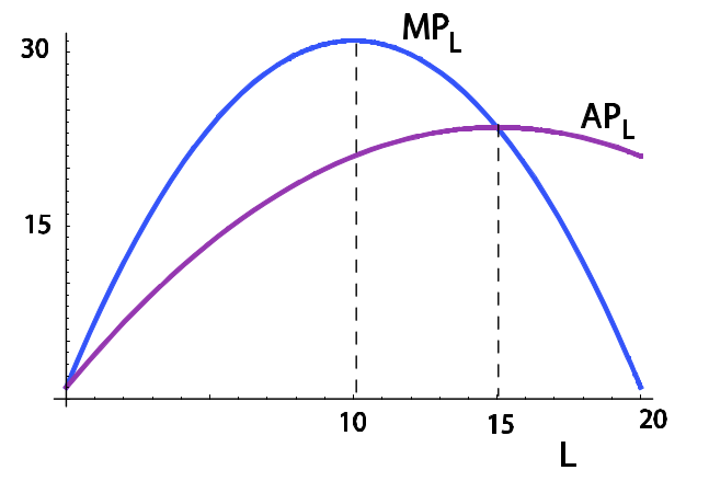
Marginal and average product

The marginal product of labour is simply the extra output by raising labour input at the margin while holding other inputs constant, given by:

MP L = ∂f (K, L)/ ∂L

Similarly, the marginal product of capital is given by:

MP K = ∂f (K, L)/ ∂K

We will assume that beyond some level of an input marginal product is diminishing. In other words, beyond some level of labour (which could be zero), MP L is decreasing in labour, and beyond some level of capital MP K is decreasing in capital. In the region with diminishing marginal product, we have:

∂^2f(K, L)/∂L^2 < 0

and:

∂^2f(K, L)/∂K^2 < 0.

The average product of labour is given by:

APL = Q/L

You can define the average product of capital similarly.

The average product rises if the average is below the marginal and falls if the average is above the marginal. At low levels of output, the marginal product is higher than the average product, and then eventually it decreases. Once it crosses below the average product, the average product falls. It follows that the crossing point is the highest point on the average curve.

5.5 The short run: one variable factor

In the short run, capital is fixed, only labour is variable. How should a firm choose how much labour to hire, and how does the level of hiring vary when the wage rate varies? We consider the input choice by a firm assuming that the firm buys inputs from a competitive market for inputs so that the firm takes the input prices as given in making decisions about how much of any input to buy.

With this in mind, the choice of labour input can be derived as follows. If the firm hires one extra unit of labour, its output rises by MP L . One extra unit of output raises revenue by MR L . Thus the extra revenue from employing one extra unit of labour is given by the marginal revenue product of labour:

MRP_L = MR_L × MP_L.

On the other hand, one extra unit of labour costs w (i.e. w is the marginal cost of labour). Thus the profit-maximising level is given by MRP_L = w.

The firm maximises profit given by: P(Q) f(Kfix, L) - wL - rKfix

where Kfix is the fixed level of K in the short run, and where Q = f(K, L). Differentiating where K with respect to L, we get:

P'(Q) ∂Q/∂L f + P (Q)f L − w = 0.

Since ∂Q/∂L = f L , we have: f L P 0 (Q) f + P (Q) = w.

Again, because f (K, L) = Q, this can be written as: f L P 0 (Q) Q + P (Q) = w.

Now, total revenue is P (Q) Q. So marginal revenue is P 0 (Q) Q + P (Q). Therefore, the
equation above is simply:

MP L × MR L = w.

Note that for a competitive firm, price is given and does not vary with firm output. Therefore, P 0 (Q) = 0, and the optimal labour hire equation becomes:

Pf_L = w

or price times marginal product equals the wage rate.

How does demand for labour change as the wage rate varies in the short run? Note that the marginal product of labour decreases with labour. Marginal revenue decreases as output increases, and output increases as labour increases. Therefore, as labour increases, MR falls. For a competitive firm MR is constant at price P . Thus either both MR and MP fall as labour increases (imperfect competition) or MR is constant (at price P ) while MP falls for competitive firms. Therefore, MRP falls as labour increases. It follows that if the wage rate falls, more labour is hired.

5.6 The long run: both factors are variable

With two variable factors (typically this would be the case in the long run), we can represent the production function by its level curves. An isoquant traces out the different combinations of K and L that produce a given level of output. Analogously to an indifference curve, the slope of an isoquant is given by the marginal rate of technical substitution (MRTS). The marginal rate of technical substitution of L for K is the amount by which capital can be reduced if the firm hires one extra unit of labour. Analogously to an indifference curve:

MRTS_LK = MP_L / MP_K

Analogously to an indifference curve, we assume that as L increases, MRTS_LK decreases, giving an isoquant the familiar convex shape. If Q 0 is the output along an isoquant, then convexity means that the set of combinations of K and L producing Q_0 or more is a convex set.

Suppose we scale up all inputs by a positive factor t. If output scales up by t as well, we say that the production function exhibits constant returns to scale. If output scales up by less than t, we have decreasing returns to scale.

Optimal long-run input choice

We consider the input choice by a firm assuming that the firm buys inputs from a competitive market for inputs so that the firm takes the input prices as given in making decisions about how much of any input to buy. We must minimise total costs wL + rK subject to the constraint that we produce Q 0
units, i.e. f (K, L) = Q_0.

First, set up the Lagrangian:
LG = wL + rK + λ(Q 0 − f (K, L))

The first-order conditions for a constrained minimum are:
∂LG/∂L = w − λ (∂f/∂L) = 0
∂LG/∂K = r − λ (∂f/∂K) = 0
∂LG/∂λ = Q_0 − f = 0.

From the first two first-order conditions, we get:
w/r = ((∂f / ∂LG) / (∂f /∂K)) = = MRTS_LK

These first-order conditions are not sufficient to guarantee a minimum. However, as under utility maximisation, the second-order condition for a minimum is satisfied so long as we have diminishing MRTS.

5.7 Cost curves

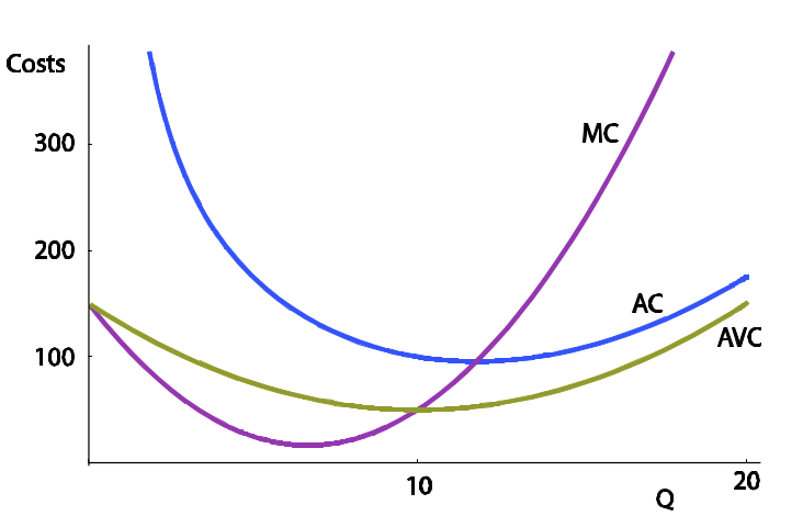
Marginal cost and average cost

Suppose TC(Q) is the total cost function for a firm. Then the marginal cost is:

MC = dTC(Q)/dQ

and the average cost is:

AC = TC(Q)/Q

It follows that if AC has a U-shape, MC must pass through the minimum point. Before this point, MC is lower than AC so AC falls, and after this point MC is above AC so AC rises.

Fixed costs and sunk costs

Fixed costs must be incurred to set up a firm. Some types of fixed costs cannot be recovered even if the firm stops production or goes out of business. Buildings and plants can be resold, but the money spent on advertising the firm’s brand name is sunk, as is the cost incurred in printing stationery.

In the short run, capital is fixed, but labour is variable. Thus there are two categories of
costs: fixed costs, F , and variable costs, VC(Q). We have:

TC(Q) = F + VC(Q).

Therefore:

AC(Q) = F/Q + VC(Q)/Q

The first component is the average fixed cost, and the second is average variable cost.

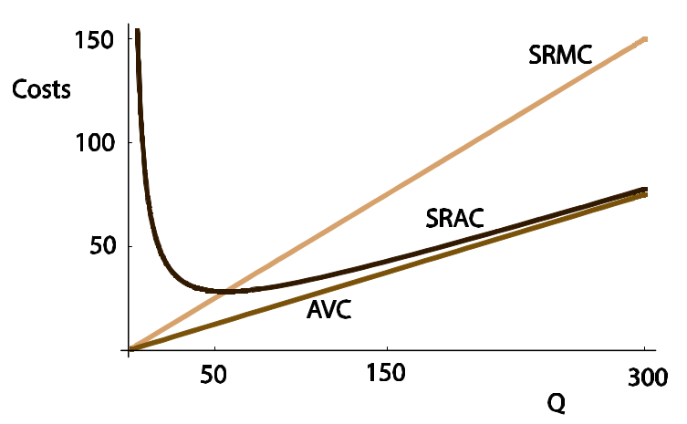
Long run

In the long run, all factors are variable, and the optimal input mix is chosen according to the long-run optimisation rule derived previously. Since capital can be varied in the long run, short-run costs are at least as high as the long-run costs, and if in the short run the firm chooses anything other than the capital size associated with the lowest long-run average costs, short-run costs are strictly higher.

The long-run average cost curve (LRAC) is an envelope of the short-run average cost curves (SRACs). Note that the long-run average cost is lower than the minimum short-run average cost over the region where the firm experiences increasing returns to scale. This is the region where the LRAC is falling. Similarly, over the region where the LRAC is increasing, the firm experiences decreasing returns to
scale and, again, the LRAC is lower than the minimum of the SRAC. For the ‘right’ long-run plant size, the minimum point of the SRAC is also the minimum point of the LRAC. Note also that the LRMC is flatter, i.e. more elastic, compared to the SRMC.

If in the long run a firm experiences increasing returns to scale at low levels of output, but decreasing returns at higher levels of output, the long-run average cost is U-shaped, and the long-run MC cuts this from below at the lowest point. However, if the firm experiences constant returns to scale, the long-run average cost curve is a horizontal line at the level of the fixed long-run average cost. In this case LRAC and LRMC are the same.

5.8 Profit maximisation

The profit of a firm is given by revenue minus cost: π = P (Q) Q − C(Q). This is maximised at the quantity where marginal revenue equals marginal cost:

(d/dQ)(P(Q)Q) - (dC(Q)/dQ) - 0

For a price-taking firm, the price P does not depend on output, so d(P Q)/dQ = P , and
profit is maximised at the output where P = MC.

Profit-maximising output
The firm must set MR equal to MC to determine the profit-maximising output level Q^∗ .

Shut-down decision

Once Q ∗ is decided, the firm must see if it is worth producing at Q ∗ .

• In the short run, a firm continues to operate even if revenues do not cover all costs. If fixed costs on equipment such as plants and machinery have been incurred, this cannot be altered in the short run. So the short-run shut-down decision pays no attention to fixed costs and only considers if the firm is covering its variable costs. The firm should continue to operate so long as it covers its variable costs. In other words, the firm shuts down production in the short run
if PQ < VC, or P < AVC.

• In the long run all factors are variable. Therefore, the firm shuts down if it cannot cover all its costs even at the minimum level of LRAC. In other words, a firm shuts down in the long run if:
P < LRAC_min

Reading: Nicholson, W., Synder, C., Intermediate Microeconomics and its application (eleventh edition), South-Western, Cengage Learning, 2010

"The laws and conditions of production partake of the character of physical truths. There is nothing arbitrary about them."
J. S. Mill, Principles of Political Economy, 1848

Chapter 6: Production

Because economists are interested in the choices that firms make to accomplish their goals, they
have developed a rather abstract model of production. In this model, the relationship between
inputs and outputs is formalized by a production function of the form

q = f(K, L, M)

where q represents the output of a particular good during a period, K represents the machine (that is, capital) use during the period, L represents hours of labor input, and M represents raw materials used.

Firm Any organization that turns inputs into outputs
Production function: The mathematical relationship between inputs and outputs.
p215-216

We simplify the production function here by assuming that the firm’s production
depends on only two inputs: capital (K) and labor (L).

q = f(K,L)

The decision to focus on capital and labor is for convenience only.
p216

Marginal product" The additional output that can be produced by adding one more unit of a particular input while holding all other inputs constant.

For our two principal inputs of capital and labor, the marginal product of labor (MP_L) is the extra output obtained by employing one more worker while holding the level of capital equipment constant. Similarly, the marginal product of capital (MP_K) is the extra output obtained by using one more machine while holding the number of workers constant.
p218

When people talk about the productivity of workers, they usually do not have in mind the economist’s notion of marginal product. Rather, they tend to think in terms of ‘‘output per worker.’’
p219

The concept of marginal product itself may sometimes be difficult to apply because of the ceteris paribus assumption used in its definition... But, in the real world, that is not how new hiring would likely occur. Rather, additional hiring would probably also necessitate adding additional equipment.

Isoquant map: A contour map of a firm’s production function.
Isoquant: A curve that shows the various combinations of inputs that will produce the same amount of
output.
p221

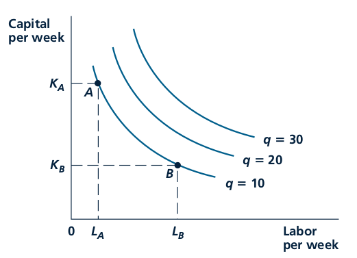
Isoquants record the alternative combinations of inputs that can be used to produce a
given level of output. The slope of these curves shows the rate at which L can be
substituted for K while keeping output constant. The negative of this slope is called the
(marginal) rate of technical substitution (RTS). In the figure, the RTS is positive, and it is
diminishing for increasing inputs of labor.

Marginal rate of technical substitution (RTS): The amount by which one input can be reduced
when one more unit of another input is added while holding output constant. The negative of
the slope of an isoquant.
p222

The isoquants in Figure 6.2 are drawn not only with negative slopes (as they should be) but also as convex curves. Along any one of the curves, the RTS is diminishing. For a high ratio of K to L, the RTS is a large positive number, indicating that a great deal of capital can be given up if one more unit of labor is employed. On the other hand, when a lot of labor is already being used, the RTS is low, signifying that only a small amount of capital can be traded for an additional unit of labor if output is to be held constant. This shape seems intuitively reasonable: The more labor (relative to capital) that is used, the less able labor is to replace capital in production. A diminishing RTS shows that use of a particular input can be pushed too far. Firms will not want to use ‘‘only labor’’ or ‘‘only machines’’ to produce a given level of output.

Returns to scale : The rate at which output increases in response to proportional increases in
all inputs.
p224

A production function is said to exhibit constant returns to scale if a doubling of all inputs results in a precise doubling of output. If a doubling of all inputs yields less than a doubling of output, the production function is said to exhibit decreasing returns to scale. If a doubling of all inputs results in more than a doubling of output, the production function exhibits increasing returns to scale.
p226

Another important characteristic of a production function is how ‘‘easily’’ capital can be substituted for labor, or, more generally, how any one input can be substituted for another. This characteristic depends primarily on the shape of a single isoquant. So far we have assumed that a given output level can be produced with a variety of different input mixes—that is, we assumed firms could substitute labor for capital while keeping output constant. How easily that substitution can be
accomplished may, of course, vary.

Fixed-proportions: production function A production function in which the inputs must be used in a fixed ratio to one another.
p229

Technical progress: A shift in the production function that allows a given output level to be
produced using fewer inputs.
p231

The RTS Is a Slope
Students sometimes confuse the slope of an isoquant with the amounts of inputs being used. The
reason we look at the RTS is to study the wisdom of changing input levels (while holding output
constant). One way to keep a focus on this question is to always think about moving counterclockwise
along an isoquant, adding one unit of labor input (shown on the horizontal axis) at a time. As we do this, the slope of the isoquant will change, and it is this changing rate of trade-off that is directly relevant to the firm’s hiring decision.
p237

Chapter 7: Costs

There are at least three different concepts of costs encountered in economics: opportunity cost, accounting cost, and economic cost. For economists, the most general of these is opportunity cost (sometimes called social cost).

Opportunity cost: The cost of a good as measured by the alternative uses that are forgone by producing the good.

Accounting cost: The concept that inputs cost what was paid for them.

Economic cost: The amount required to keep an input in its present use; the amount that it would be worth in its next best alternative use

Wage rate (w): The cost of hiring one worker for one hour.
p244

Sunk cost: Expenditure that once made cannot be recovered.

Rental rate (v): The cost of hiring one machine for one hour.
p245

Total costs = TC = wL + vK

Economic profit = Total Revenues - Total Costs = Pq - wL - vK
= Pf(K, L) - wL - vK

Economic profits (pi) The difference between a firm’s total revenues and its total economic costs.

To minimize the cost of producing q 1 , a firm should choose that point on the q 1 isoquant that has the lowest cost. That is, it should explore all feasible input combinations to find the cheapest one. p247

This will require the firm to choose that input combination for which the marginal rate of technical substitution (RTS) of L for K is equal to the ratio of the inputs’ costs, w/v
p247-248

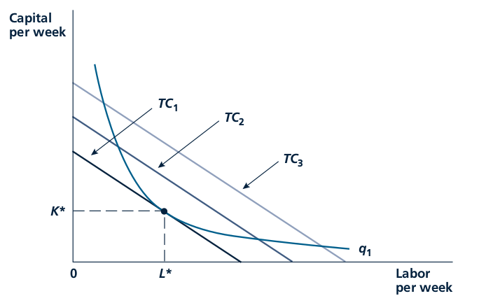
A firm is assumed to choose capital (K) and labor (L) to minimize total costs. The condition
for this minimization is that the rate at which L can be substituted for K (while keeping q 1⁄4
q 1 ) should be equal to the rate at which these inputs can be traded in the market. In other
words, the RTS (of L for K) should be set equal to the price ratio w/v. This tangency is shown
here in that costs are minimized at TC 1 by choosing inputs K* and L*.
p249

Expansion path: The set of cost-minimizing input combinations a firm will choose to produce various levels of output (when the prices of inputs are held constant).
p250

Average cost: Total cost divided by output; a common measure of cost per unit. AC = TC/q
p253

Marginal cost: The additional cost of producing one more unit of output. MC = delta TC/delta q
p254

Short run: The period of time in which a firm must consider some inputs to be fixed in making its decisions.

Long run: The period of time in which a firm may consider all of its inputs to be variable in making its decisions.

Fixed costs: Costs associated with inputs that are fixed in the short run.

Variable costs: Costs associated with inputs that can be varied in the short run.
p257

Economies of scope: Reductions in the costs of one product of a multiproduct firm when the output of another product is increased.
p264

Production Functions Determine the Shape of Cost Curves
The shapes of a firm’s cost curves are not arbitrary. They relate in very specific ways to the firm’s
underlying production function. For example, if the production function exhibits constant returns to
scale, both long-run average and long-run marginal costs will be constant no matter what output is.
Similarly, if some inputs are held constant in the short run, diminishing returns to those inputs that are variable will results in average and marginal costs increasing as output expands. Too often, students rush to draw a set of cost curves without stopping to think about what the production function looks like.
p268