4.1 Introduction

In many economic situations agents must act strategically by taking into account the behaviour of others. Game theory provides a set of tools that enables you to analyse such situations in a logically coherent manner. For each concept introduced, you should try to understand why it makes sense as a tool of analysis and (this is much harder) try to see what its shortcomings might be. This is not the right place to ask questions such as ‘what is the policy-relevance of this concept?’. The concepts you come across here are just tools, and that is the spirit in which you should learn them. As you will see, some of these concepts are used later in this course (as well as in a variety of other economics courses that you might encounter later) to analyse certain types of economic interactions.

The chapter aims to familiarise you with a subset of basic game theory tools that are used extensively in modern microeconomic theory. The chapter aims to cover simultaneous-move games as well as sequential-move games, followed by an analysis of the repeated Prisoners’ Dilemma game.

By the end of this chapter, the Essential reading and activities, you should be able to:

* analyse simultaneous-move games using dominant strategies or by eliminating dominated strategies either once or in an iterative fashion
* calculate Nash equilibria in pure strategies as well as Nash equilibria in mixed strategies in simultaneous-move games
* explain why Nash equilibrium is the central solution concept and explain the importance of proving existence
* specify strategies in extensive-form games
* analyse Nash equilibria in extensive-form games
* explain the idea of refining Nash equilibria in extensive-form games using backward induction and subgame perfection
* analyse the infinitely-repeated Prisoners’ Dilemma game with discounting and analyse collusive equilibria using trigger strategies
* explain the multiplicity of equilibria in repeated games and state the folk theorem for the Prisoners’ Dilemma game.

4.3 Simultaneous-move or normal-form games

A simultaneous-move game (also known as a normal-form game) requires three elements. First, a set of players. Second, each player must have a set of strategies. Once each player chooses a strategy from their strategy set, we have a strategy profile. The third element of a game is a payoff function for each player. A payoff function for any player is defined over the set of strategy profiles. For each strategy profile, each player gets a payoff.

We write this in a convenient matrix form (known as the normal form) as follows. The first number in each cell is the payoff of player 1 and the second number is the payoff of player 2. Note that player 1 chooses rows and player 2 chooses columns. It is sometimes useful to write the strategy profile (s 1 , s 2 , . . . , s n ) as (s i , s −i ), where s −i is the profile of strategies of all players other than player i. So: s −i = (s 1 , s 2 , . . . , s i−1 , s i+i . . . . , s n ) With this notation, we can write the payoff of player i as u i (s i , s −i ).

Dominant and dominated strategies

A player has a strategy that gives a higher payoff compared to other strategies irrespective of the strategy choices of others. Such a strategy is called a dominant strategy. If a player has a dominant strategy, his problem is simple: he should clearly play that strategy. If each player has a dominant strategy, the equilibrium of the game is obvious: each player plays his own dominant strategy.

Consider the following game. Each player has two strategies C (cooperate) and D (defect, which means not to cooperate). There are 4 possible strategy profiles and each profile generates a payoff for each player. The first number in each cell is the payoff of player 1 and the second number is the payoff of player 2. Again, note that player 1 chooses the row that is being played and player 2 chooses the column that is being played.

 
		Player 2
		C	D
Player 1 C	2,2	0,3
	 D	3,0	1,1

Here each player has a dominant strategy, D. This is the well-known Prisoners’ Dilemma game. Rational players, playing in rational self-interest, get locked into a ominant-strategy equilibrium that gives a lower payoff compared to the situation where both players cooperate.

Strategy s ∗ i of player i is a dominant strategy if:

u i (s ∗ i , s −i ) > u i (s i , s −i ) for all s i different from s ∗ i and for all s −i .

That is, s ∗ i performs better than any other strategy of player i no matter what others are playing.

Even if a player does not have a dominant strategy, he might have one or more dominated strategies. A dominated strategy for i is a strategy of i (say s i ) that yields a lower payoff compared to another strategy (say s 0 i ) irrespective of what others are playing. In other words, the payoff of i from playing s i is always (i.e. under all possible choices of other players) lower than the payoff from playing s 0 i . Since s i is a dominated strategy, i would never play this strategy. Thus we can eliminate dominated strategies.

Here is another example of a dominance solvable game. We find the equilibrium of this
game by iteratively eliminating dominated strategies.

		Player 2
		Left	Middle	Right
	Top	4,3	2,7	0,4
Player1	Middle	5,5	5,-1	-4,-2
	Bottom	3,5	1,5	-1,6

We can eliminate dominated strategies iteratively as follows.

1. For player 1, Bottom is dominated by Top. Eliminate Bottom.
2. In the remaining game, for player 2, Right is dominated by Middle. Eliminate Right.
3. In the remaining game, for player 1, Top is dominated by Middle. Eliminate Top.
4. In the remaining game, for player 2, Middle is dominated by Left. Eliminate Middle.

This gives us (Middle, Left) as the unique equilibrium.

However, for many games the above criteria of dominance do not allow us to find an equilibrium. Players might not have dominant strategies; moreover none of the strategies of any player might be dominated. The problem with dominance criteria is that they apply only to some games. For games that do not have dominant or dominated strategies, the idea of deriving an equilibrium using dominance arguments does not work.

If we want to derive an equilibrium that does not rely on specific features such as dominance, we need a concept of equilibrium that applies generally to all games. As we show below, a Nash equilibrium (named after the mathematician John Nash) is indeed such a solution concept.

We start by analysing Nash equilibrium under pure strategies. Later we introduce mixed strategies. We then note that one can prove an existence result: all games have at least one Nash equilibrium (in either pure or mixed strategies). This is why Nash equilibrium is the central solution concept in game theory.

Nash equilibrium in pure strategies
A strategy profile (s ∗ i , s ∗−i ) is a Nash equilibrium if for each player i:
u i (s ∗ i , s ∗−i ) ≥ u i (s i , s ∗−i ) for all strategies s i in the set S i .

To find out the Nash equilibrium we must look for the mutual best responses in terms of payoff.

				Player 2
			A 2	B 2	C 2
		A 1	3, 1	1, 3	4, 2
Player 1	B 1	1, 0	3, 1	3, 0
		C 1	2, 3	2, 0	3, 2

Best options for Player 1 are A1, B1, A1, for A2, B2, C2
Best options for Player 2 are B2, B2, A2, for A1, B1, C1

Nash equilibrium is not necessarily unique. There can be multiple pure strategy Nash equilibria.

Mixed strategy
A mixed strategy s i is a probability distribution over the set of (pure) strategies.

Once we include mixed strategies in the set of strategies, we have the following
existence theorem, proved by John Nash in 1951.

Existence theorem
Every game with a finite number of players and finite strategy sets has at least one Nash equilibrium.

4.4 Sequential-move or extensive-form games

Let us now consider sequential move games. In this case, we need to draw a game tree to depict the sequence of actions. Games depicted in such a way are also known as extensive-form games.

To start with, we assume that each player can observe the moves of players who act before them. First, we need to understand the difference between actions and strategies in such games. Once we clarify this, we show how to derive Nash equilibria. Finally, we propose a refinement of Nash equilibrium: subgame perfect Nash equilibrium. In games where all moves of previous players can be observed, subgame perfect Nash equilibria can be derived by backward induction.

The notion of a strategy is fairly straightforward in a normal form game. However, for an extensive-form game, it is a little bit more complicated. A strategy in an extensive form game is a complete plan of actions. In other words, a strategy for player i must specify an action at every node at which i can possibly move.

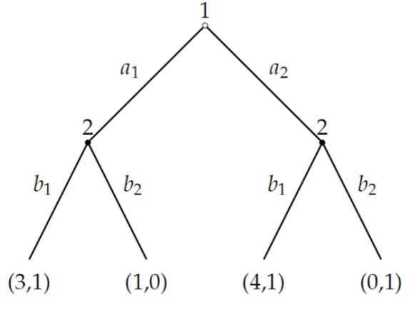
The strategy set of player 2 is {(b 1 b 1 ), (b 1 b 2 ), (b 2 b 1 ), (b 2 b 2 )}

Imperfect information: information sets

Consider the extensive-form game introduced at the start of this section. Suppose at the time of making a decision, player 2 does not know what strategy player 1 has chosen. Since player 2 does not know what player 1 has chosen, at the time of taking an action player 2 does not know whether he is at the left node or at the right node. To capture this situation of imperfect information in our game-tree, we say that the two decision nodes of player 2 are in an information set.

Note that player 2 knows he is at the information set (after player 1 moves), but does not know where he is in the information set (i.e. he does not know what player 1 has chosen). Since player 2 cannot distinguish between the two nodes inside his information set, he cannot take different actions at the two nodes. Therefore, the strategy set of 2 is simply {b 1 , b 2 }

4.5 Incredible threats in Nash equilibria and subgame perfection

Nash equilibrium allows for some strategies by later movers that seem like threats which are incredible. In Nash equilibrium, a player is just supposed to take a best response to the other players’ strategy choices – so the way Nash equilibrium is constructed does not allow the player to ignore certain strategy choices of others as incredible. Once we look at some examples of the problem, we will try to see whether we can refine the set of Nash equilibria to eliminate the possibility of such threats (i.e. come up with extra conditions that an equilibrium must satisfy so that equilibria which depend on incredible threats will not satisfy these extra conditions).

A subgame is a part of a game that starts from a node which is a singleton (i.e. a subgame does not start at an information set), and includes all successors of that node. If one node in an information set belongs to a subgame, so do all other nodes in that information set. In other words, you cannot cut an information set so that only part of it belongs to a subgame. That would clearly alter the information structure of the game, which is not allowed.

We can now define a subgame perfect equilibrium.

Subgame perfect Nash equilibrium
A strategy combination is a subgame perfect Nash equilibrium (SPNE) if:
it is a Nash equilibrium of the whole game
it induces a Nash equilibrium in every subgame.

It should be clear from the definition that the set of subgame perfect equilibria is a refinement of the set of Nash equilibria.

In perfect information games (recall that, in a game of perfect information, each player knows all past moves of other players), this is easy. Subgame perfect Nash equilibria can be derived simply by solving backwards, i.e. by using backward induction.

Backward induction need not work under imperfect information: you cannot fold backwards when you come up against an information set. Indeed, this is why the concept of a subgame perfect Nash equilibrium is more general compared to backward induction.

4.6 Repeated Prisoners’ Dilemma

In a one-shot game, rational players simply play their dominant strategies. So (D, D) is the only possible equilibrium. Suppose the game is repeated. Can we say something about the behaviour of players in such ‘supergames’ that differs from the behaviour in the one-shot game?

While the logic is inescapable, actual behaviour in laboratory settings differs from this. Faced with a large finite number of repetitions, players do cooperate for a while at least. Therefore, it is our modelling that is at fault (or, the players are being "irrational"). To escape from the logic of backward induction, we can assume that when a game is repeated many times, players play them as if the games are infinitely repeated. In that case, we must apply forward-looking logic as there is no last period from which to fold backwards.

Options:
Cooperation through trigger strategies
Start by playing C (that is, cooperate at the very first period, when there is no
history yet).
In period t > 1:
• if (C, C) was played last period, play C
• if anything else was played last period, play D.

Folk theorem
The Folk theorem is the following claim. Consider any pair of payoffs (π 1 , π 2 ) such
that π i > 1 for i = 1, 2. Any such payoff can be supported as an equilibrium payoff for
high enough

Reading: Nicholson, W., Synder, C., Intermediate Microeconomics and its application (eleventh edition), South-Western, Cengage Learning, 2010

Chapter 5: Game Theory

A central assumption in this text is that people make the best choices they can given their objectives... Many situations are more complicated in that they involve strategic interaction. The best one person can do may often depend on what another does. p175

One branch of game theory, called cooperative game theory, assumes the group of players reaches an outcome that is best for the group as a whole... We focus on noncooperative game theory for several reasons. Self-interested behavior does not always lead to an outcome that is best for the players as a group.. , and such outcomes are interesting and practically relevant... self-interested behavior is the natural extension of our analysis of single-player decision problems in earlier chapters to a strategic setting... one can analyze attempts to cooperate using noncooperative game theory.. noncooperative game theory is more widely used by economists..cooperative game theory has proved useful to model bargaining games and political processes. p176

Game theory models seek to portray complex strategic situations in a simplified setting... Any strategic situation can be modeled as game by specifying four basic elements: (1) players, (2) strategies, (3) payoffs, and (4) information. p176

Each decision maker in a game is called a player.
A player’s choice in a game is called a strategy.
The returns to the players at the conclusion of the game are called payoffs.
What players know when they make their moves, called their information. p176-177

Best response: A strategy that produces the highest payoff among all possible strategies for a
player given what the other player is doing.

Nash equilibrium: A set of strategies, one for each player, that are each best responses against one another.

In a two-player game, a set of strategies (a*, b*) is a Nash equilibrium if a* is player A’s best response against b* and b* is player B’s best response against a*. A Nash equilibrium is stable in the sense that no player has an incentive to deviate unilaterally to some other strategy.
p178

Normal form: Representation of a game using a payoff matrix.
Extensive form: Representation of a game as a tree.
p180

Specify Equilibrium Strategies
The temptation is to say that the Nash equilibrium is (3,3). This is not technically correct. Recall that the definition of the Nash equilibrium involves a set of strategies, so it is proper to refer to the Nash equilibrium in the Prisoners’ Dilemma as ‘‘both players choose Confess.’’ True, each outcome corresponds to unique payoffs in this game, so there is little confusion in referring to an equilibrium by the associated payoffs rather than strategies. However, we will come across games later in the chapter in which different outcomes have the same payoffs, so referring to equilibria by payoffs leads to ambiguity.

Dominant strategy: Best response to all of the other player’s strategies.
p182

Pure strategy: A single action played with certainty.
Mixed strategy: Randomly selecting from several possible actions.
p184

Indifferent among Random Actions
In any mixed-strategy equilibrium, players must be indifferent between the actions that are played with positive probability. If a player strictly preferred one action over another, the player would want to put all of the probability on the preferred action and none on the other action.
p186

Best-response function: Function giving the payoff-maximizing choice for one player for each of a continuum of strategies of the other player. p189

Focal point: Logical outcome on which to coordinate, based on information outside of the game. p192

Proper subgame: Part of the game tree including an initial decision not connected to another in an oval and everything branching out below it.

Subgame-perfect equilibrium: Strategies that form a Nash equilibrium on every proper subgame.
p197

Backward induction: Solving for equilibrium by working backward from the end of the game to the beginning.
p199

Stage game: Simple game that is played repeatedly.
p200

Trigger strategy: Strategy in a repeated game where the player stops cooperating in order to punish another player’s break with cooperation.
p202

Incomplete information: Some players have information about the game that others do not.
p208