7.1 Introduction

Previously, we have studied competitive equilibrium in specific markets. This chapter now introduces the idea of an economy-wide general equilibrium. The analysis of competitive markets allowed us to evaluate welfare in a specific market. A general equilibrium allows an evaluation of welfare in the entire economy. To simplify the exposition and make the main ideas clear, we focus extensively on an exchange economy. We consider the conditions for a general equilibrium and discuss the two welfare theorems in detail. Later on, we assume that there is one agent (or a representative agent) in an economy to introduce production in a simple setting.

* construct an Edgeworth box and depict the contract curve, the set of possible equilibrium exchanges given an endowment point, and depict the equilibrium price ratio and allocation
* derive algebraically the contract curve, the equilibrium price ratio and allocation explain that only relative prices matter
* explain the importance of establishing existence
* state and provide an informal proof outline for the first welfare theorem in the context of an exchange economy with two agents and two goods as well as in the context of an economy with production
* discuss the policy implications of the first welfare theorem and understand the situations in which the theorem might not apply
* state and provide an informal proof outline for the second welfare theorem in the context of an exchange economy with two agents and two goods
* discuss the policy implications of the second welfare theorem and understand the situations in which the theorem might not apply
* derive the equilibrium conditions in an economy with production

The chapter starts by covering general equilibrium in an exchange economy. Next, the chapter remarks briefly on the existence of equilibrium before moving on to considering the content and implications of the two welfare theorems. Finally, the chapter outlines general equilibrium in an economy, including production.

7.3 General equilibrium in an exchange economy

An exchange economy is characterised by endowments and preferences of all individuals. We first give a general definition of the general equilibrium (or exchange equilibrium) for such an economy, sometimes called the Walrasian equilibrium. Suppose there are I > 1 agents and n > 1 goods. Let x_j^i denote the demand by agent i for good j, and let e_j^i be agent i’s endowment of good j. The utility function of agent i is

u_i (x_1^i ... x_n^i).

The budget constraint of i is:

p_1 x_1^i + p_2 x_2^i + ... + p_n x_n^i = p_1 e_1^i + p_2 e_2^i + ... + p_n e_n^i.

General equilibrium
A general equilibrium for a pure exchange economy consists of prices (p_1 , . . . , p_n ) and
quantities ((x_1^1 , . . . , x_n^1), . . . , (x_1^I , . . . , x_n^I )) such that:
* at the given prices, for each i, the bundle (x_1^i , . . . , x_n^i ) maximises utility of agent
i, subject to the agent’s budget constraint.
* all markets clear, i.e. for each market j, total demand equals total supply:
Sum x_j^i = Sum e_j^i

The final consumption bundles of agents are together known as the equilibrium allocation.

General equilibrium in such a two-person exchange economy can be usefully studied
using an Edgeworth box diagram. You should be able to construct such a diagram
and depict the set of Pareto efficient outcomes (the contract curve), be able to identify
the possible set of Pareto-improving trades given initial endowments, be able to identify
the possible set of equilibrium exchanges, and be able to show the equilibrium price
ratio and equilibrium allocation.

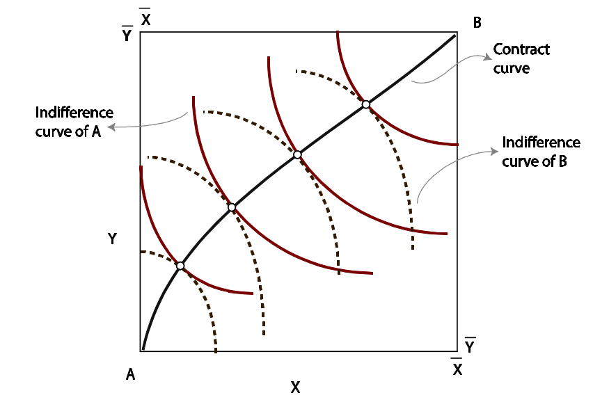
The contract curve traces out the Pareto efficient allocations in the Edgeworth box. These are points of tangency between the indifference curves of A and B. Once we reach such a point of tangency, it is impossible to make one agent better off without making the other agent worse off. Therefore, if through trading a point on the contract curve is reached, no further trade is possible. Conversely, if trading has reached any point not on the contract curve, further Pareto-improving trades are possible.

We can also derive the set of Pareto-efficient allocations algebraically. To do this, we
solve the following problem:

max X_A Y_A X_B Y_B u_A(X_A, Y_A)

subject to the following constraints:
u_B (X_B , Y_B ) = ū
X_A + X_B = X̄
Y_A + Y_B = Ȳ .

Therefore, we have: MRS_A = MRS_B

The set of allocations that are possible to achieve by trading starting from the initial allocation, E. These allocations give at least as much utility as the endowment to either agent. In other words, each point in this set of allocations (excluding E itself and the other crossing point between the indifference curves) Pareto dominates E.

We can now introduce prices. The slope of the price line is −P Y /P X . Trading can take
place along any such price line. Any arbitrary price line cannot guarantee an equilibrium. The property that the price line must satisfy in order to produce an equilibrium. It must be tangent to the indifference curves of both agents. This can of course happen only on the contract curve, since this also requires the indifference curves themselves to be tangent to each other.

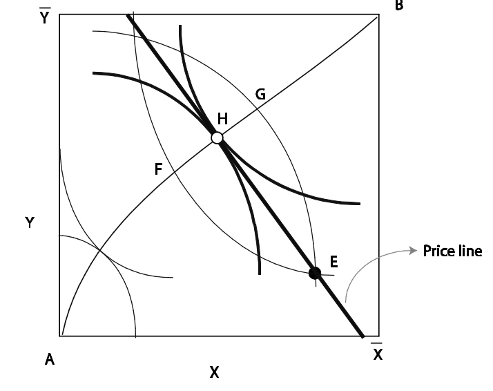
Note that the price line and, therefore, the equilibrium allocation would remain unchanged if all prices are multiplied by the same positive number. Essentially, in a general equilibrium we can only determine ‘relative’ prices.

7.5 Uniqueness

General equilibrium in an economy need not be unique.

7.6 Welfare theorems

Pareto efficient allocation
An allocation of resources is Pareto efficient if it is not possible to reallocate resources to make one person better off without making someone else worse off.

The terms Pareto optimal, Pareto efficient, and efficient are used interchangeably. Note that the notion of efficiency in economics says nothing about equity. Contract curves include points where one consumer gets a very high utility while another gets a very low utility. Later, when we study monopoly, you will see that if a monopolist can extract the entire surplus, the market outcome is efficient, while if the monopolist cannot do so the outcome is typically inefficient even though consumers do receive some surplus.

The first theorem of welfare economics

The first theorem of welfare economics says that the competitive equilibrium is Pareto efficient. In other words, the process of decentralised decision-making by agents and the equilibrating force of market prices together ensure that there are no gains from trade left unexploited. Starting from any equilibrium allocation, if we want to make any one agent better off, we can do that only by making someone else worse off.

The first theorem of welfare economics applies in a very general setting, and is an absolute blockbuster. This remarkable result is fundamental to our understanding of markets.

The first thing it tells us is about the remarkable ability of the price mechanism to eliminate inefficiencies. Even though markets are a conglomeration of a large number of agents trying to maximise their own utility without paying attention to what others might be doing, the price mechanism creates the right incentives for agents to exploit every trading opportunity. Wherever any opportunity for efficiency-enhancing trade is left, prices will be such that agents will have the incentive to exploit these opportunities.

You should be able to show the result easily in a two-agent two-good exchange economy. Looking at Edgeworth box diagrams, you should be able to see that it is impossible to make anyone better off without making the other agent worse off.

While this theorem is fundamental to our understanding of economics, you should also be aware that the argument can be taken too far. To see the flaw in this doctrine, you need to understand the concept of a ‘market failure’. A market failure occurs when the equilibrium in a market involves some deadweight loss, i.e. the equilibrium admits some degree of inefficiency. The theory of general equilibrium that we described above assumes away such problems, but these are relevant in manyall situations.

To summarise, the first welfare theorem is one of the most (if not the most) important results in economics. It provides a benchmark against which to judge the social welfare from any market outcome. There are various instances where market outcomes do admit inefficiency, in which case there is a role for policy.

Finally, note that policy itself can be subject to problems. Governments themselves might sometimes serve special interests, and in such cases interventions need not be efficiency-enhancing. Along with market failures, you should also keep in mind the possibility of such government failures.

The second theorem of welfare economics

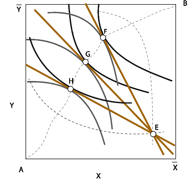
The first welfare theorem says that any general equilibrium allocation is efficient. The second theorem makes a sort of reverse statement. It says that if all agents have convex preferences, any efficient allocation can be obtained as an equilibrium if we can suitably change the initial endowment point.

This is easy to see in a two-agent two-good economy. As you know, efficient allocations are points on the contract curve. Let us pick an arbitrary point H on the contract curve. This is a point of tangency between indifference curves of the two agents, i.e. the indifference curves have the same slope at H. So long as preferences are convex (diminishing MRS), both agents would choose H as the
utility-maximising point.

What does this mean? To see this, suppose we want a particular distribution of welfare among agents. Can we achieve this distribution without wasting resources? That is, can we reallocate resources in an efficient manner? The theorem shows that the answer to this question is yes.

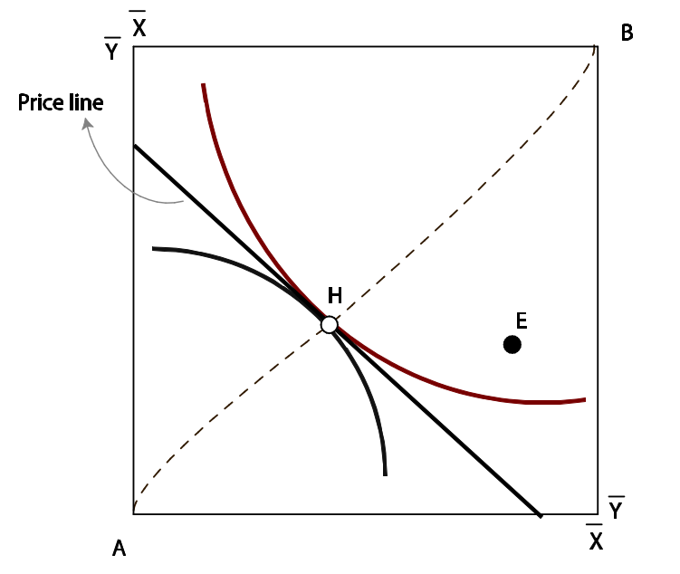
H is a Pareto efficient allocation, but on the price line that has the same slope as the common slope of the indifference curves at H, the optimal choice of agent A is not H, but G. Therefore, H is a Pareto efficient allocation but it cannot be supported as an equilibrium. In other words, if the government wanted to achieve a redistribution to the point H and redistributed endowments suitably, the economy would not stay at point H as the market process would move it away.

Next, consider the question of the redistribution of resources. How do we do this? In an ideal world we would use lump-sum taxes and transfers. Indeed, if we could use lump-sum taxes quite easily in practice, this theorem would spell out the right type of policy to achieve different welfare distributions. However, lump-sum taxes are difficult to impose in practice. A lump-sum tax is a tax imposed on something that an agent cannot change. A tax on labour endowment or any type of earned income is distortionary – any such tax would lead agents to change how much labour they supply or how much effort they invest in earning. Furthermore, even if you could find a lump-sum tax (such as a poll tax), people might not fully trust the government to make use of the proceeds in the right manner. This might make such a tax politically unpalatable. These problems with lump-sum taxes limit the force of the second welfare theorem as a tool for the real world.

7.7 Production

Consider an economy with two goods (x and y) and one agent in society. This sort of an economy is often referred to as a ‘Robinson Crusoe’ economy. In an economy with many identical agents you can simply solve the problem of a ‘representative agent’. This is why analysing single-agent economies makes sense. Single-agent economies are used often by macroeconomists in building a micro-foundation for macroeconomic models.

The utility function of Robinson is given by u(x, y).

The production possibility frontier shows the combinations of x and y that can be produced using the resources available in the economy.

The slope of the frontier at any point shows how much y we need to give up to obtain one extra unit of x. This is called the marginal rate of transformation (MRT). Typically, the MRT is increasing as we raise x (and lower y).

A society’s production possibility frontier comes in the implicit form T (x, y) = 0. (For example, if the production possibility frontier is y = √(c − x^2), we can write it in the implicit form as x^2 + y^2 − c = 0.)

Reading: Nicholson, W., Synder, C., Intermediate Microeconomics and its application (eleventh edition), South-Western, Cengage Learning, 2010

Chapter 10: General Equilibrium and Welfare

General equilibrium model: An economic model of a complete system of markets.

Partial equilibrium model: An economic model of a single market.

In all of these many markets, a few basic principles are assumed to hold:
* All individuals and firms take prices as given—they are price takers.
* All individuals maximize utility.
* All firms maximize profits.
* All individuals and firms are fully informed; there are no transactions costs, and there is no uncertainty.

p346

Economically efficient allocation of resources: An allocation of resources in which the sum of consumer and producer surplus is maximized. Reflects the best (utility-maximizing) use of scarce resources.

p348

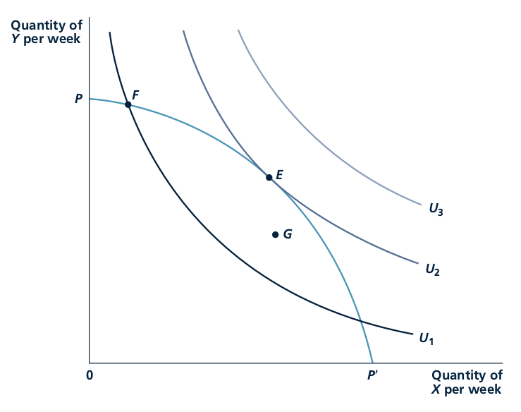
The efficient allocation shown at point E in Figure 10.2 is characterized by a tangency between the production possibility frontier and consumer’s indifference curve. The increasingly steep slope of the frontier shows that X becomes relatively more costly as its production is increased. On the other hand, the slope of an indifference curve shows how people are willing to trade one good for another in consumption (the marginal rate of substitution). That slope flattens as people consume more X because they seek balance in what they have. The tangency in Figure 10.2 therefore shows that one sign of efficiency is that the relative opportunity costs of goods in production should equal the rate at which people are willing to trade these goods for each other. In that way, an efficient allocation ties together technical information about relative costs from the supply side of the market with information about preferences from the demand side. If these slopes were not equal (say at point F) the allocation of resources would be inefficient (utility would be U 1 instead of U 2 ).

p350

First theorem of welfare economics: A perfectly competitive price system will bring about an economically efficient allocation of efficient allocation of resources.

p351

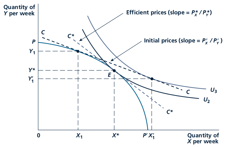
With an arbitrary initial price ratio, firms will produce X 1 , Y 1 ; the economy’s budget constraint will be given by line CC. With this budget constraint, individuals demand X 1 0 , Y 1 , that is, there is an excess demand for good X (X 1 0 X 1 ) and an excess supply of good Y (Y 1 Y 1 0 ). The workings of the market will move these prices toward their equilibrium levels P X^* ,P Y^* . At those prices, society’s budget constraint will be given by the line C*C*, and supply and demand will be in equilibrium. The combination X*, Y* of goods will be chosen, and this allocation is efficient.

p352

Perfect Substitutes When goods are perfect substitutes, individual’s marginal rates of substitution between the goods will determine relative prices. This is the only price ratio that can prevail in equilibrium because at any other price ratio, individuals would choose to consume only one of the goods.

p354

Slopes and Tangencies Determine Efficient Allocations
Efficiency in economics relates to the trade-offs that firms and individuals make. These trade-offs are captured by the slope of the production possibility frontier and by the slopes of individuals’ indifference curves. The efficient points cannot be found by dealing with quantities alone. This is a mistake beginning students often make—they try to find solutions without ever looking at trade-off rates (slopes). This approach ‘‘worked’’ in our first example because you just had to find the point of the production possibility frontier where X 1⁄4 Y. But, even in that case, it was impossible to calculate relative prices without knowing the slope of the frontier at this point. In more complicated cases, it will be generally impossible even to find an efficient allocation without carefully considering the trade-off rates involved.

p355

Showing that perfect competition is economically efficient depends crucially on all of the assumptions that underlie the competitive model. Several conditions that may prevent markets from generating such an efficient allocation.

Imperfect competition: A market situation in which buyers or sellers have some influence on the prices of goods or services.

Externality: The effect of one party’s economic activities on another party that is not taken into account by the price system.

Public goods: Goods that are both nonexclusive and nonrival.

Imperfect Information: Throughout our discussion of the connection between perfect competition and economic efficiency, we have been implicitly assuming that the economic actors involved are fully informed.

p356-p357

A primary problem with developing an accepted definition of ‘‘fair’’ or ‘‘unfair’’ allocations of resources is that not everyone agrees as to what the concept means.

p360

Issues about equity can best be illustrated with a graphic device called the Edgeworth box diagram. In this diagram, a box is used that has dimensions given by the total quantities of two goods available (we’ll call these goods simply X and Y). The horizontal dimension of the box represents the total quantity of X available, whereas the vertical height of the box is the total quantity of Y.

p360-361

Pareto efficient allocation : An allocation of available resources in which no mutually beneficial trading opportunities are unexploited. That is, an allocation in which no one person can be made better off without someone else being made worse off.

Contract curve : The set of efficient allocations of the existing goods in an exchange situation. Points off that curve are necessarily inefficient, since individuals can be made unambiguously better off by moving to the curve

p362

Initial endowments: The initial holdings of goods from which trading begins.

p363

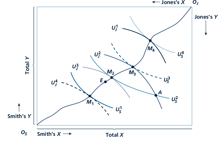
This Edgeworth box diagram for exchange is taken from Figure 10.5. Point E represents a
‘‘fair’’ sharing of the available goods (assuming that can be defined). If individuals’ initial
endowments are at point A, voluntary transactions cannot be relied on to reach point E
since such an allocation makes Smith worse off than at A.
p364