8.1 Introduction

Previously, we analysed competitive markets. In these markets firms are price-takers, and the market price is determined by the interaction of industry supply and market demand, a process over which no single firm has any control. In this chapter we develop the model of the opposite market structure – one where the supply side consists of a single firm. The other dimension in which the analysis differs is that a monopolist is relatively unconstrained in choosing its pricing strategy. Instead of choosing a single price, it can choose different prices across different identifiable groups or markets, and also charge a fee to give a consumer access to purchasing. We analyse the consequences of these pricing schemes. Finally, certain markets naturally lend themselves to a monopoly structure. Such natural monopolies also present unique regulatory challenges. We analyse the problem of natural monopolies and explain the regulatory problems.

We aim to explain how profit maximisation by a monopoly firm leads to a distortion in the market, and try to understand the policies that try to address this problem. We also aim to analyse different price discrimination schemes and try to understand what impact they have on profits and efficiency loss. Overall, our main focus here is on the design of pricing schemes as well as the design of regulatory schemes to eliminate or limit any deadweight loss.

* derive the marginal revenue curve associated with any demand curve
* explain the relationship between marginal revenue and price elasticity of demand as well as Lerner’s index
* analyse the profit-maximising choice by the monopolist and the associated deadweight loss
* analyse the role of regulatory policies
* analyse a variety of price discrimination policies that a monopolist can employ
* analyse the structure of natural monopoly and the regulatory problem in this case.

The chapter analyses the profit-maximising outcome for a monopolist and the resulting deadweight loss. Next, the chapter analyses a variety of price discrimination schemes. Finally, the chapter introduces the problem of natural monopoly.

8.3 Properties of marginal revenue

You should study carefully the properties of marginal revenue (MR) detailed in N&S Sections 8.3 and 8.4. You should understand how to derive the MR curve for a downward-sloping demand curve (in this case, the average revenue is falling which implies marginal revenue is below average revenue).

You should also understand the relationship between MR and price elasticity. This can be derived as follows:

MR = (d/dQ)(P(Q)Q) = (dP/dQ)Q+P = (1 + (Q/P))(dP/dQ)= P (1+1/ε)

where ε < 0. To make this fact explicit, it might be useful to rewrite this using the
absolute value of price elasticity:

We have the following:

* If ε < −1 (i.e. |ε| > 1), demand is elastic and MR > 0.
* If ε = −1 (i.e. |ε| = 1), demand is unit elastic and MR = 0.
* If ε > −1 (i.e. |ε| < 1), demand is inelastic and MR < 0.

Figure 8.1 below shows the relationship between elasticity and MR for the linear demand curve P = 10 − Q.

8.4 Profit maximisation and deadweight loss

You should know how to derive the profit-maximising solution for a monopolist and how to depict this in a diagram. You should be able to calculate the deadweight loss at the monopoly optimum.

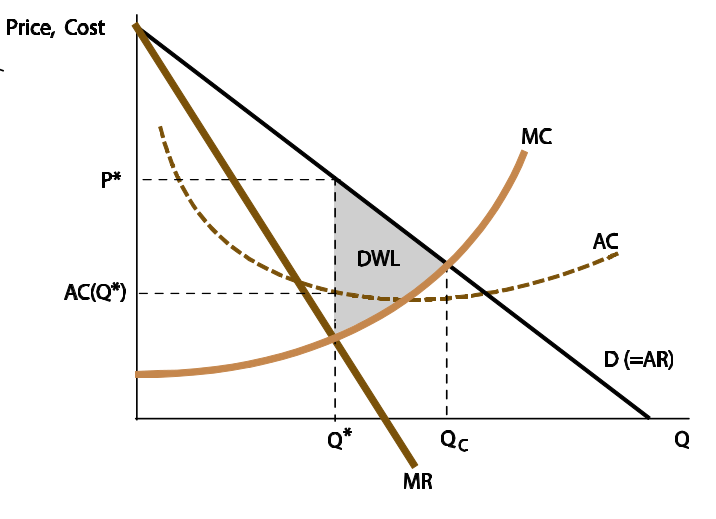
A monopolist’s profit is T R − T C, and this is maximised at the quantity where MR = MC. Figure 8.2 shows the profit-maximising quantity and price. Note that the profit at the optimum is given by (P − AC(Q ∗ )) Q ∗

Figure 8.2 also shows the deadweight loss under monopoly. Note that Q C is the competitive output where P = MC. What is the source of the deadweight loss under monopoly? Essentially, a monopolist tries to maximise profit by restricting output. This causes the output to be lower than the competitive output at which there would be no deadweight loss.

Profit maximisation under a linear demand curve

Consider the linear demand curve shown. Note that at MR = 0 we have |ε| = 1. Therefore, for any positive MC, the optimal output-price combination occurs at the left of the unit elasticity point. At all such points demand is elastic. It follows that for a linear demand curve, the monopolist always produces at the elastic part of the curve.

Regulation

Since a monopoly gives rise to an efficiency loss, the question of regulation becomes relevant. You should be able to understand and analyse regulatory strategies to reduce monopoly deadweight loss. One way to regulate a monopoly is to specify the price that a monopolist can charge. By restricting price to the level P = MC(Q C ), the regulator can eliminate deadweight loss. Another policy is to encourage new entry in the industry so that there is increased competition, which reduces the price towards marginal cost and reduces deadweight loss.

The Lerner index

Since profit is maximised at MR = MC, at the optimum point:

MC = P(1+1/ε)

which implies:

(P-MC)/P = -(1/ε) = 1/|ε|

The left-hand side is known as the Lerner index, which is a measure of the monopoly power of a firm. For a competitive firm, P = MC so that the Lerner index is 0. If MC is 0 or P is infinity, the Lerner index is 1, which is its maximum value. For a monopolist, it lies between 0 and 1 and rises as demand becomes less elastic.

8.5 Price discrimination

A monopoly firm need not charge a single price to all customers. There are a variety of ways in which it can practise price discrimination. There is perfect price discrimination, market separation, two-part tariffs, as well as a variety of non-linear pricing schemes. A durable good monopolist faces competition with its own future self, which affects pricing.

8.6 Natural monopoly

In some industries, there is a large fixed cost but a relatively low marginal cost of production. For example, it is costly to set up a gas, electricity, water or telephone network, but once this fixed cost (installing pipes, cables etc.) is incurred, the cost of connecting an additional subscriber is close to zero. In such cases, the long-run average cost curve falls over the relevant range of output. In such cases, it is efficient to have a single firm because multiple firms would only replicate the fixed cost unnecessarily. In other words, a single firm can produce the market output at a lower cost compared to several firms. A monopoly with this characteristic is called a natural monopoly. Utilities are often granted such status by governments because they are thought to be natural monopolies. Figure 8.3 shows the situation faced by a natural monopoly.

A standard monopolist can be regulated by setting the regulated price equal to marginal cost at the efficient quantity. However, such an approach runs into difficulty here. Since the AC is falling, the MC is below the AC, implying that if the regulated price is set equal to the MC, the monopolist would incur a loss and quit rather than produce. As you can see from Figure 8.3, pricing at the MC implies a loss for the monopolist. The government then must give a lump-sum subsidy to the monopolist to cover the losses. However, governments typically do not want to be in a position to subsidise a monopolist forever. In that case, the government can regulate the monopolist by setting the price equal to average cost. This implies that the deadweight loss is not fully eliminated, as shown in Figure 8.3. Alternatively, the monopolist might be allowed to charge a higher price to some consumers and a lower price to others. A multi-product monopolist might be allowed to make a profit on some products while making a loss on others through marginal cost pricing, while making a zero profit overall.

Reading: Nicholson, W., Synder, C., Intermediate Microeconomics and its application (eleventh edition), South-Western, Cengage Learning, 2010

Chapter 11: Monopoly

A market is described as a monopoly if it has only one supplier. This single firm faces the entire market demand curve. Using its knowledge of this demand curve, the monopoly makes a decision on how much to produce. Unlike the single competitive firm’s output decision (which has no effect on market price), the monopoly output decision will completely determine the good’s price.

Barriers to entry are the source of all monopoly power. There are two general types of barriers to entry: technical barriers and legal barriers.

p378

A primary technical barrier to entry is that the production of the good in question exhibits decreasing average cost over a wide range of output levels. That is, relatively large-scale firms are more efficient than small ones. In this situation, one firm finds it profitable to drive others out of the industry by price cutting... Because this barrier to entry arises naturally as a result of the technology of production, the monopoly created is sometimes called a natural monopoly.

p378-379

Many pure monopolies are created as a matter of law rather than as a result of economic conditions. One important example of a government-granted mono- poly position is the legal protection provided by a patent. A second example of a legally created monopoly is the awarding of an exclusive franchise or license to serve a market. These are awarded in cases of public utility.

p379

As in any firm, a profit-maximizing monopoly will choose to produce that output level for which marginal revenue is equal to marginal cost. Because the monopoly, in contrast to a perfectly competitive firm, faces a downward-sloping demand curve for its product [as opposed to horizontal], marginal revenue is less than market price. To sell an additional unit, the monopoly must lower its price on all units to be sold in order to generate the extra demand necessary to find a taker for this marginal unit. In equating marginal revenue to marginal cost, the monopoly produces an output level for which price exceeds marginal cost. This feature of monopoly pricing is the primary reason for the negative effect of monopoly on resource allocation.

p380

No single curve can capture the monopolist’s supply decision. The monopolist bases its supply decision on marginal revenue rather than demand directly, and marginal revenue depends on the shape of the demand curve (that is, both the slope of the demand curve as well as its level). Therefore, in the monopoly case, we refer to the firm’s supply ‘‘decision’’ rather than supply ‘‘curve.’’

p381

Monopolies pose several problems for any economy. Here, we look at two specific complaints: first, monopolies produce too little output; and second, the high prices they charge end up redistributing wealth from consumers to the ‘‘fat cat’’ firm owners.

p382

A perfectly competitive industry would produce output level Q* at a price of P*. A monopolist would opt for Q** at a price of P **. Consumer expenditures and productive inputs worth AEQ*Q** are reallocated into the production of other goods. Consumer surplus equal to P**BAP* is transferred into monopoly profits. There is a deadweight loss given by BEA.

p383

So far in this chapter we have assumed that a monopoly sells all its output at one price. The firm was assumed to be unwilling or unable to adopt different prices for different buyers of its product. There are two consequences of such a policy. First, as we illustrated in the previous section, the monopoly must forsake some transactions that would in fact be mutually beneficial if they could be conducted at a lower price.... The existence of both of these areas of untapped opportunities suggests that a monopoly has the possibility of increasing its profits even more by practicing price discrimination—that is, by selling its output at different prices to different buyers. In this section, we examine some of these possibilities.

p388-389

Perfect price discrimination: Selling each unit of output for the highest price obtainable. Extracts all of the consumer surplus available in a given market.

p389

Perhaps somewhat paradoxically, this perfect price discrimination scheme results in an equilibrium that is economically efficient. Because trading proceeds to the point at which price is equal to marginal cost, there are no further unexploited trading opportunities available in this marketplace. Of course, this solution requires that the monopoly knows a great deal about the buyers of its output in order to determine how much each is willing to pay. It also requires that no further trading occur in this good in order to prevent those who buy it at a low price from reselling to those who would have paid the most to the monopoly. The pricing scheme will not work for goods like toasters or concert tickets, which may easily be resold; but, for some services, such as medical office visits or personalized financial or legal planning, providers may have the required monopoly power and may know their buyers well enough to approximate such a scheme.

A second way that a monopoly firm may be able to practice price discrimination is to separate its potential customers into two or more categories and to charge different amounts in these markets. If buyers cannot shift their purchasing from one market to another in response to price differences, this practice may increase profits over what is obtainable under a single-price policy.

p390

The price discrimination strategy in the previous section requires the monopolist to be able to distinguish the two markets by observation. As long as consumers cannot easily travel between them, different geographic markets are trivial to distinguish by observation. In cases in which the monopolist cannot separate consumers into different markets by observation, it can practice a different form of price discrimination. It can offer different amounts of the good at different per-unit prices. Nonlinear pricing may be a profitable strategy if each consumer potentially has demand for several units of the good. This is the case with coffee, for example, because consumers typically do not just drink one ounce but may drink a variable amount... The monopolist can increase profits by fine-tuning the nonlinear pricing scheme to take account of variation in consumer valuations of different units of the good.

Nonlinear pricing: Schedule of quantities sold at different per-unit prices.

p393

The monopolist could also use other strategies that have a similar effect to reducing durability. An automobile manufacturer could lease the cars instead of selling them. This would force the consumers to return to the car market more often (after the lease is up rather than after the car breaks down). Software firms could come out with more frequent upgrades. In the art market, artists sometimes use the unique strategy of destroying the stone after producing a limited quantity of numbered lithographs, a sure commitment to maintain scarcity and high prices over time.

There are basically two solutions to minimizing the allocational harm caused by monopolies: (1) make markets more competitive, and (2) regulate price in the monopoly market. In general, economists favor the first of these. Actions that loosen entry barriers (such as eliminating restrictive licensing requirements) can sharply reduce the power of a monopoly to control its prices. Similarly, antitrust laws can be used to reduce the power of monopoly firms to raise entry barriers on their own. Because direct price regulation can be problematic (as we shall see), pro-competitive solutions will generally work better. In the case of a natural monopoly, however, that will not be the case. When average costs fall over the entire range of output, the cost-minimizing solution is to have only a single firm provide the good. Production by several firms would, by definition, be inefficient because it would involve extra costs. Hence, in a natural monopoly situation, direct price regulation may be the only option. How to achieve this regulation is an important subject in applied economics. The utility, communications, and transportation industries are all subject to price regulation in many countries.

p400

Natural monopolies, by definition, exhibit decreasing average costs over a broad range of output levels. The cost curves for such a firm might look like those shown in Figure 11.8. In the absence of regulation, the monopoly would produce output level Q A and receive a price of P A for its product.
Profits in this situation are given by the rectangle P A ABC. A regulatory agency might set a price of P R for this monopoly. At this price, Q R is demanded, and the marginal cost of producing this output level is also P R . Consequently, marginal cost pricing has been achieved. Unfortunately, because of the declining nature of the firm’s cost curves, the price P R (1⁄4 marginal cost) falls below average costs. With this regulated price, the monopoly must operate at a loss given by area GFEP R . Since no firm can operate indefinitely at a loss, this poses a dilemma for the regulatory agency: Either it must abandon its goal of marginal cost pricing, or the government must subsidize the monopoly forever.

p401

One way out of the marginal cost pricing dilemma is a two-part pricing system. Under this system, the monopoly is permitted to charge some users a high price while maintaining a low price for ‘‘marginal’’ users. In this way, the demanders paying the high price in effect subsidize the losses of the low-price customers.

p402