9.1 Introduction

When an industry comprises of a few firms, the nature of competition is very different from that under perfect competition. In trying to maximise profit, a firm must not only take into account the impact of its own supply on the market price, but must also account for the strategic responses of other firms. We have already analysed this type of interaction when we studied game theory, and identified Nash equilibrium as the central solution concept. Recall that a Nash equilibrium is a mutual best response: given what others are doing, each firm must play a best response. We now use this solution concept to analyse the outcome under quantity and price competition.

In this chapter we aim to analyse the market structure when there are a few firms in the market. We aim to analyse the nature of strategic interaction among firms when firms compete in quantities as well as under price competition. We aim to understand the oligopoly models of Cournot competition with and without collusion, Stackelberg leadership, Bertrand competition with and without collusion, as well as price competition with differentiated products under simultaneous and sequential price-setting.

* derive the Nash equilibrium in a Cournot game
* analyse collusion in a Cournot game
* analyse Stackelberg leadership
* derive the Nash equilibrium in a Bertrand game
* analyse collusion in a Bertrand game
* derive the Nash equilibrium in a Bertrand game with differentiated products
* derive the equilibrium in the game of sequential price-setting with differentiated products.

9.3 Cournot competition

This is a game with continuous (rather than discrete) strategy sets. The inverse demand function in an industry is given by p = a − bQ, where p is the market price, Q is the aggregate supply in the market, and a, b are positive constants. There are n > 1 firms in this industry, and each firm produces the output at a marginal cost c, with c < a. First, suppose n = 2. Let us compute the Nash equilibrium of this game, which is also called the Cournot equilibrium, or the Cournot–Nash equilibrium.

The profit of firm 1 is:

Π1(q1 , q2 ) = (p − c)q 1 = (a − bQ − c)q 1 = (a − bq 1 − bq 2 − c)q 1 .

The first-order condition for maximising profit is ∂Π 1 /∂q 1 = 0 which implies:

q1 = (a-c)/2b - (q2/2)

This is the best response function of firm 1 (also called the reaction function of firm 1).
After optimisation, we impose symmetry: q 1 = q 2 = q. This implies:

q = (a-c-bq)/2b

Here we imposed symmetry after optimisation. However, this method does not work if the firms are not symmetric. Suppose the marginal costs are c 1 and c 2 . In this case, you must derive the two best response functions, and then solve two simultaneous equations for q 1 and q 2 .

Note that an increase in c 1 reduces the equilibrium output of firm 1, but raises that of firm 2. Graphically, the best response function of firm 1 moves inwards, so that the Nash equilibrium point slides up along the best response function of firm 2.

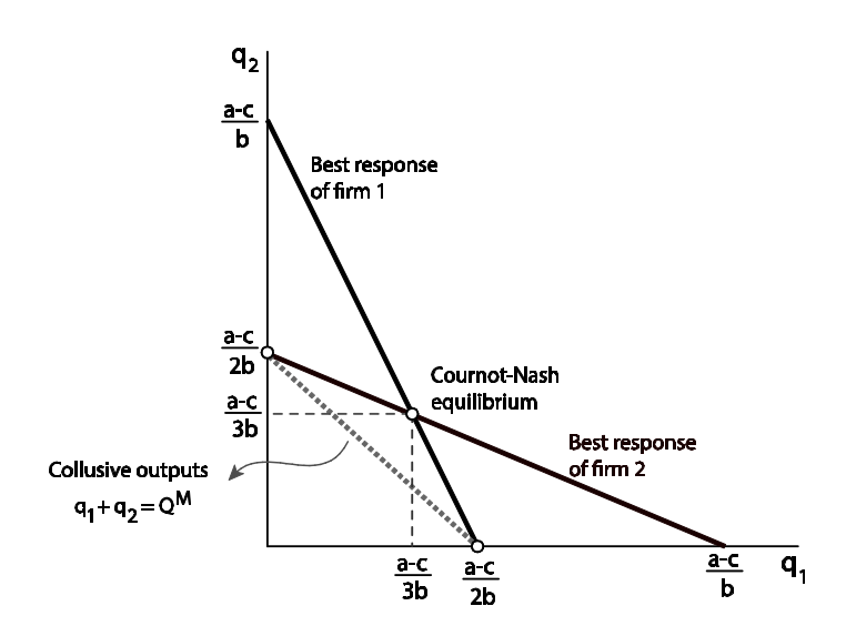
Collusion

Suppose the firms could collude by some means. Let us calculate the output, price and profit in this case. Let Q M = q 1 + q 2 be the collusive output. The joint profit is:

Π^M (Q^M ) = (a − bQ^M − c)Q^M .

The market price is: p^M = a − b × (a − c)/2b = (a + c)/2

The total profit is: Π^M = ( (a+c)/2) - c)((a-c)/2b) = (a-c)^2/4b > 2Π^D

The monopoly outcome cannot be sustained in a one-shot game – the best response of firm 1 to any q 2 is to produce more than the collusive output.

However, in an infinitely-repeated game, the collusive output can be sustained as the outcome of an equilibrium if the players are sufficiently patient. You already know this result from the theory of repeated games.

Such a strategy is called a ‘trigger’ strategy since a deviation by any single firm triggers non-cooperation in all future periods. We denote the total duopoly Cournot–Nash equilibrium quantity by Q^D , i.e. Q^D = q_1^∗ + q_2^∗

The payoff of each firm under collusion is necessarily higher than that under Cournot competition), the expression on the right-hand side is less than 1. Therefore, for δ high enough (close enough to 1), the above inequality is satisfied for all i, and for such values of δ, collusion can be sustained.

Cournot with n > 2 firms

The Cournot outcome converges to the competitive outcome as n goes to infinity.

Stackelberg leadership

Instead of being a simultaneous-move game, if firms play an extensive-form game with one firm choosing quantity before another, the firm choosing first is the Stackelberg leader, while the second mover is the follower.

The second mover will choose a best response to the first mover’s quantity. Therefore, the second mover will always be on his best response function. Knowing this, at the first stage, the first mover simply chooses the best point on the second mover’s best response function.

Compared to the Cournot–Nash outputs, the first mover produces more and, given this, the second
mover’s best response is to produce a lower output.

If the leader chooses the Cournot–Nash quantity, the follower’s best response would also be to choose the Cournot–Nash quantity. However, the leader can do even better given the freedom to choose any point on the follower’s best response function. Therefore, the Stackelberg leader must earn a greater profit compared to that under Cournot competition.

9.4 Bertrand competition

If firms compete in prices, and each firm can serve the whole market, the only equilibrium is p = c. You should be able to go through the detailed argument to establish this. Bertrand competition results in the competitive outcome, a result sometimes referred to as the Bertrand paradox.

Collusion

If firms play an infinitely-repeated game, and are patient enough, we know from game theory that they can sustain a high collusive price.

Bertrand competition with product differentiation

Two firms have differentiated products so that the demand functions are as follows:

q_1 = α − P_1 + P_2 and q_2 = α − P_2 + P_1

Why is this a model of differentiated products? Note that the demand for the product of firm 1, say, does not vanish if P_1 > P_2 . In this case, the demand for firm 2’s product will be higher, but firm 2 will not take over the entire market. The underlying idea here is that firms have different products that are substitutable, but not completely so. As firm 1’s price increases, some of the customers (who only consider firm 1’s product to be marginally better than firm 2’s) will switch to buying firm 2’s product – lowering demand for firm 1 and raising that for firm 2.

Sequential pricing

In the Stackelberg model, we studied the outcome under quantity competition when firms move sequentially. Here, let us study the same market structure with pricing. Suppose firm 1 moves first, followed by firm 2. In the second stage, firm 2 will always be on its best response function. Therefore, firm 1 chooses the best point on firm 2’s best response function in the first stage.

In the Stackelberg equilibrium, the leader gets the higher profit. Here, the follower benefits more than the leader. The reason is that higher prices set by firm 1 at stage 1 are advantageous to firm 2, as a higher price set by firm 1 means that the environment faced by firm 2 is less competitive. Note that the price charged by firm 1 is higher than that under the simultaneous-move game. This means that in the sequential-move game firm 2 faces a less competitive environment compared to the simultaneous-move game.

Reading: Nicholson, W., Synder, C., Intermediate Microeconomics and its application (eleventh edition), South-Western, Cengage Learning, 2010

Chapter 12: Imperfect Competition

A hallmark of an imperfectly competitive market is the presence of few firms but more than one, in which case the market is called an oligopoly.

p408

It is difficult to predict exactly the possible outcomes for prices when there are few firms; prices depend on how aggressively firms compete, which in turn depends on which strategic variables firms choose, how much information firms have about rivals, and how often firms interact with each other in the market. The Bertrand model—which we will study in detail later in the chapter—in which identical firms choose prices simultaneously in their one meeting in the market, has a Nash equilibrium at point C in Figure 12.1. This figure assumes that marginal cost (and average cost) is constant for all output levels. Even though there may be only two firms in the market, in this equilibrium they behave as if they were perfectly competitive, setting price equal to marginal cost and earning zero profit.

At the other extreme, firms as a group may act as a cartel, recognizing that they can affect price and coordinate their decisions. Indeed, they may be able to act as a perfect cartel, achieving the highest possible profits, namely, the profit a monopoly would earn in the market.

p409

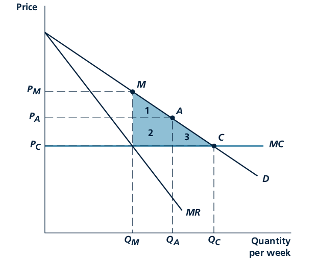
Market equilibrium under imperfect competition can occur at many points on the demand curve. In this figure, which assumes that marginal costs are constant over all output ranges, the equilibrium of the Bertrand game occurs at point C, also corresponding to the perfectly competitive outcome. The perfect-cartel outcome occurs at point M, also corresponding to the monopoly outcome. Many solutions may occur between points M and C, depending on the specific assumptions made about how firms compete.

p410

Cournot model: An oligopoly model in which firms simultaneously choose quantities.

p411

Lerner Index
Asking where an industry falls between points C and M in Figure 12.1 is really just asking how competitive the industry is. The most widely used measure is called the Lerner index (L), which equals the percentage markup of price over marginal cost:

L = P - MC / P

The index is expressed as a percentage to remove the units in which the product is measured). If the industry is perfectly competitive, the Lerner index equals zero since price equals marginal cost. For the monopoly/perfect cartel outcome, one can show that the Lerner index is related to the elasticity
of market demand; 1 more precisely, the inverse of the abso lute value of the elasticity,

L = 1 / abs e_Q1P

ranging from close to zero for very elastic demand curves to extremely high numbers for very inelastic demand curves.

However price data can be readily obtained just by looking at an advertisement or visiting a store. Unfortunately, data on marginal costs are not readily available. Firms often jealously guard cost information as being competitively sensitive.

p411

Nash Equilibrium in the Cournot Model

For a pair of quantities, q A and q B , to be a Nash equilibrium, q A must be a best response to q B and vice versa. We therefore begin by computing the best-response function for firm A. Its best-response function tells us the value of q A that maximizes A’s profit given for each possible choice q B by firm B.

p414

Comparisons and Antitrust Considerations

The Nash equilibrium of the Cournot model is somewhere between perfect competition and monopoly. That equilibrium price and industry profit in the Cournot model is above the perfectly competitive level and below the monopoly level; industry output is below the perfectly competitive level and above the monopoly level. The firms manage not to compete away all the profits as in perfect competition. But the firms do not do as well as a monopoly would, either.

p415

GAMES WITH CONTINUOUS ACTIONS
The methods used to solve the Cournot model are similar to those used to solve the Tragedy of the
Commons from Chapter 5. In fact, except for the interpretation of the players’ identities (shepherds
versus spring-water producers) and actions (number of sheep versus thousands of gallons of spring
water), the two games are exactly the same. The reader can verify that the equilibrium in both involves a choice of 40 units for each player.

The Cournot model can be relatively easily extended to cases involving more complex demand and cost assumptions or to situations involving three or more firms. As the number of firms grows large, it can be shown that the Nash equilibrium approaches the competitive case, with price approaching marginal cost. The ease with which the model can be extended, together with the fact that it produces what people think is a realistic outcome for most markets (that is, an outcome between perfect competition and monopoly), has made the Cournot model a work-horse for economists.

p416

Bertrand model: An oligopoly model in which firms simultaneously choose prices.

We next turn to the Bertrand model, named after the economist who first proposed it. 4 Bertrand thought that Cournot’s assumption that firms choose quantities was unrealistic, so he developed a model in which firms choose prices. In all other respects the model is the same as Cournot’s. We will see that this seemingly small change in the strategic variable from quantities in the Cournot model to prices in the Bertrand model leads to a big change in the equilibrium outcome.

The only Nash equilibrium in the Bertrand game is for both firms to charge marginal cost: P_A = P_B = c. In saying that this is the only Nash equilibrium, we are really making two statements that both need to be verified: (1) that this outcome is a Nash equilibrium, and (2) that there is no other Nash equilibrium.

p418

Bertrand Paradox

The Nash equilibrium of the Bertrand model is the same as the perfectly competitive outcome. Price is set to marginal cost, and firms earn zero profit. The result that the Nash equilibrium in the Bertrand model is the same as in perfect competition even though there are only two firms in the market is called the Bertrand Paradox. It is paradoxical that competition would be so tough with as few as two firms in the market. In one sense, the Bertrand Paradox is a general result in that we did not specify the marginal cost c or the demand curve, so the result holds for any c and any downward-sloping demand curve.

In another sense, the Bertrand Paradox is not very general; it can be undone by changing any of a number of the model’s assumptions. For example, assuming firms choose quantity rather than price leads to the Cournot game, and we saw from our analysis of the Cournot game that firms do not end up charging marginal cost and earning zero profit. The Bertrand Paradox could also be avoided by making other assumptions, including the assumption that the marginal cost is higher for one firm than another, the assumption that products are slightly differentiated rather than being perfect substitutes, or the assumption that firms engage in repeated interaction rather than one round of competition. In the next section, we will see that the Bertrand Paradox can be avoided by assuming firms have capacity constraints rather than the ability to produce an unlimited amount at constant cost c.

p419

Capacity constraint: A limit to the quantity a firm can produce given the firm’s capital and other available inputs.

The assumption that firms do not have capacity constraints is crucial for the stark result in the Bertrand model. Starting from equal prices, if a firm lowers its price slightly, its demand essentially doubles. The firm can satisfy this increased demand because it has no capacity constraints, giving firms a big incentive to undercut. If the undercutting firm could not serve all the demand at its lower price because of capacity constraints, that would leave some residual demand for the higher-priced firm, and would decrease the incentive to undercut.

p419

Comparing the Bertrand and Cournot Results

The contrast between the Bertrand and Cournot models is striking. The Bertrand model predicts competitive outcomes in a duopoly situation, whereas the Cournot model predicts prices above marginal cost and positive profits; that is, an outcome somewhere between competition and monopoly. These results suggest that actual behavior in duopoly markets may exhibit a wide variety of outcomes depending on the precise way in which competition occurs. The range of possibilities expands yet further if we add product differentiation or tacit collusion (issues we will study later in the chapter) to the model. Determining the competitiveness of a particular real-world industry is therefore a matter for careful empirical work.

p420

Economists tend to view informative advertising favorably, as a way to lower consumer search costs, increasing transparency and thus firms’ competitiveness in the market. A second type of advertising, persuasive advertising, attempts to convince consumers to buy one product rather than another close—perhaps perfect—substitute... Some economists view persuasive advertising less favorably, as a way to soften price competition by increasing apparent rather than real product differentiation.

p426

We mentioned that the Cournot and Bertrand games bear some resemblance to the Prisoners’ Dilemma in that if the firms could cooperate to restrict output or raise prices, they could increase the profits of both, just as the players in the Prisoners’ Dilemma would benefit from cooperating on being Silent. In Chapter 5 we concluded that if the Prisoners’ Dilemma were repeated an indefinite number of times, the participants can devise ways to adopt more cooperative strategic choices. A similar possibility arises with the Cournot and Bertrand games. Repetition of these games offers a mechanism for the firms to earn higher profits by pursuing a monopoly pricing policy.

p428

The contrast between the competitive results of the Bertrand model and the monopoly results of the tacit-collusion model suggests that the viability of collusion in game-theory models is very sensitive to the particular assumptions made. It was assumed that a firm can easily detect whether another has cheated. In practice, however, the deviator may cut price secretly, and other buyers may not learn about the deviation until much later. In the model, a lag in detection is similar to increasing the period length, which in turn is similar to reducing the probability, g, that the game continues (because the probability that the game ends compounds over time).

p431

Stackelberg Equilibrium: Subgame-perfect equilibrium of the sequential version of the Cournot game.

p434